Pandas の代わりに Polars を使用:パフォーマンスの深層分析
本記事は、大規模データ処理において従来の Pandas に代わる Rust ベースの Polars の性能優位性を、具体的なコーディング課題を通じて実証し、並列処理と遅延評価の技術的メリットを詳細に解説している。
キーポイント
Pandas の大規模データにおけるボトルネック
数百万行以上のデータでは、グループ化演算の遅延、中間コピーによるメモリ消費、および Python レベルのループによる非ベクトル化処理がパフォーマンスの重大な欠点となる。
Polars の技術的優位性
Rust で構築され Apache Arrow を基盤とする Polars は、並列実行と遅延評価を第一級機能として備え、クエリ計画の最適化により全 CPU コアを自動的に活用して高速化する。
実データを用いた性能比較
StrataScratch の実課題(メール活動ランクなど)を用いて両ライブラリの解決策を比較し、特に大規模データ処理における劇的な速度差とメモリ効率の向上を実証している。
ランク付けの誤解と解決策
Pandas の `rank(method='dense')` は同点の場合に同じ順位を割り当てるため、一意な順位が必要な場合は不適切です。
Polars による効率的なソートと番号付け
Polars ではソート順(総メール数降順、ユーザーID昇順)を指定し、`with_row_count` で連続した一意の順位を直接割り当てることで複雑なロジックを回避できます。
単一パスによる最適化
Polars の LazyFrame は名前変更、グループ化、ソート、行番号割り当てを一度の処理で完結させ、Pandas のような複数回のデータ反復や複雑なランク計算を不要にします。
並列処理による高速化
Polars は利用可能なすべての CPU コアに負荷を分散して集計を行うため、大規模テーブルでは Pands よりも著しく高速な処理が可能です。
重要な引用
For datasets that fit in memory, it is fast and familiar enough that switching libraries rarely crosses any programmer's mind.
Polars is a DataFrame library built in Rust on top of Apache Arrow. It was designed with parallelism and lazy evaluation as first-class features.
The correct method is 'first', which breaks ties by position in the sorted frame.
No tie-breaking logic is needed because the sort already handled it.
The Pandas solution iterates over the data twice after grouping: once to compute sizes and once to assign ranks.
On a table containing millions of email records, the use of parallel aggregation without a rank function can result in a 5–10x improvement in wall-clock time compared to the Pandas approach.
影響分析・編集コメントを表示
影響分析
この分析は、データエンジニアリングおよびデータサイエンスの実務において、パフォーマンスボトルネックを解消するための具体的な技術的移行指針を提供するものである。特に大規模データを扱う現場では、Pandas から Polars への移行が処理時間の短縮とリソースコストの削減に直結するため、業界標準のワークフロー変更に大きな影響を与える可能性がある。
編集コメント
大規模データ処理の現場では、ライブラリの選択がシステム全体のレスポンスに直結するため、この性能比較は非常に実用的な価値を持ちます。特に Rust の採用によるメモリ安全性と速度の両立は、今後の Python エコシステムにおける重要なトレンドを示唆しています。
**
# イントロダクション
過去10年間、Pandas** は Python におけるデータ処理の基盤として君臨してきました。メモリーに収まるデータセットにおいては、その速度と親しみやすさから、ライブラリを切り替えることを考えるプログラマーはほとんどいません。
しかし、数百万行規模のデータを扱うようになると、欠陥が顕在化し始めます:数秒かかるグループ化演算、RAM を消費する中間コピー、そしてベクトル化された C や Rust コードではなく Python レベルのループとして実行されるウィンドウ関数などです。
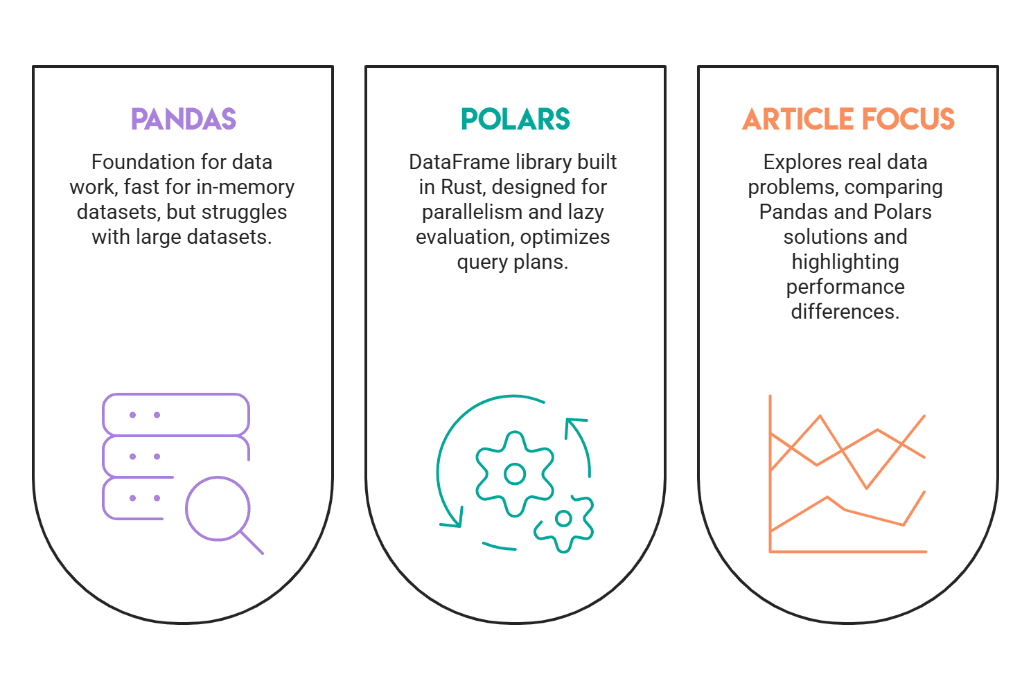
Polars は、Apache Arrow を基盤とした Rust で構築された DataFrame ライブラリです。並列処理と遅延評価が第一級機能として設計されています。Pandas は各演算を逐次的に即座に実行するのに対し、Polars はクエリプランを構築して実行前に最適化し、利用可能なすべての CPU コアでほとんどの演算を自動的に並行して実行します。
本記事では、StrataScratch コーディングプラットフォームからの実際の質問を用いた 3 つの現実的なデータ問題を取り上げます。各問題について両ライブラリの解決策を比較し、パフォーマンスの違いが最も顕著に現れる箇所を指摘します。
**
# rank() と with_row_count() の比較:アクティビティランク
この質問では、送信されたメールの総数に基づいて各ユーザーのメールアクティビティランクを見つけることが目的です。最も多くのメールを送信したユーザーにランク 1 が付与されます。結果は、送信メール数の降順でソートされ、同点の場合はアルファベット順を tiebreaker(同点処理基準)として使用し、2 人のユーザーが同じメール数を持っていても各ランクは一意である必要があります。
// データビュー
google_gmail_emails テーブルには、送信されたメールごとに 1 行が格納されており、送信者 ID (from_user)、受信者 ID (to_user)、およびメールの送信日が含まれています。以下にテーブルのプレビューを示します:
id
from_user
to_user
day
0
6edf0be4b2267df1fa
75d295377a46f83236
10
1
6edf0be4b2267df1fa
32ded68d89443e808
6
2
6edf0be4b2267df1fa
55e60cfcc9dc49c17e
10
3
6edf0be4b2267df1fa
e0e0defbb9ec47f6f7
6
4
...
...
...
314
e6088004caf0c8cc51
e6088004caf0c8cc51
5
粒度**(出力行 1 つが意味するもの):1 人のユーザー、その総メール数、および一意のアクティビティランク。
// よくある間違い
この質問は、2人のユーザーのメール数が同じであっても一意のランクを要求するものです。よくある間違いは、Pandas の rank(method='dense') メソッドを使用することです。これは同点のユーザーに同じランクを割り当ててしまいます。正しい方法は 'first' で、これはソートされたフレーム内の位置に基づいて同点を打破します。ランク付けの前に user_id についてアルファベット順にソートしているため、結果として得られるランクは一意かつ決定論的になります。
Polars の最適解では rank 関数を完全に回避しています。それぞれ降順と昇順で ["total_emails", "user_id"] でソートした後、.with_row_count("activity_rank", offset=1) クラースが 1 から始まる連続する整数を割り当てます。ソート自体が同点打破処理を行っているため、同点を打破するためのロジックは不要です。
// Solutions
1. Pandas Solution
from_user を user_id にリネームし、user でグループ化してメール数をカウントし、最初のランクを計算し、メール数降順でソートします。同点の場合はアルファベット順で打破します。
import pandas as pd
import numpy as np
google_gmail_emails = google_gmail_emails.rename(columns={"from_user": "user_id"})
result = google_gmail_emails.groupby(
    ['user_id']).size().to_frame('total_emails').reset_index()
result['activity_rank'] = result['total_emails'].rank(method='first', ascending=False)
result = result.sort_values(by=['total_emails', 'user_id'], ascending=[False, True])
2. Polars Solution
名前の変更、グループ化、ソート、行番号の割り当てを単一のパスで行う 遅延チェーン を使用します。最後に .collect() を呼び出すことで、結果がマテリアライズされます。
import polars as pl
google_gmail_emails = google_gmail_emails.rename({"from_user": "user_id"})
result = (
    google_gmail_emails.lazy()
    .group_by("user_id")
    .agg(total_emails = pl.count())
    .sort(
        by=["total_emails", "user_id"],
        descending=[True, False]
    )
    .with_row_count("activity_rank", offset=1)
    .select([
        pl.col("user_id"),
        "total_emails",
        "activity_rank"
    ])
    .collect()
)
// パフォーマンス比較
**

Pandas の解決策では、グループ化後にデータを 2 回反復処理します。1 回はサイズを計算するため、もう 1 回はランクを割り当てるためです。内部では rank(method='first') がランク配列を割り当て、argsort を用いて同点の解決を行い、書き戻しを行います。これは単一の列に対しては見た目以上にコストがかかる処理です。一方、Polars の group_by 関数は利用可能なすべての CPU コアに負荷を分散させるため、大規模なテーブルに対する集計が大幅に高速化されます。また、.with_row_count() クロースはソート後の単一の O(n) 順次パスであるため、rank 関数よりも最もコストの低い操作で置き換えることができます。数百万件のメールレコードを含むテーブルにおいて、ランク関数を使用せずに並列集計を行うことで、Pandas のアプローチと比較して実行時間(wall-clock time)が 5〜10 倍改善される可能性があります。
以下にコード出力のプレビューを示します:
user_id
total_emails
activity_rank
32ded68d89443e808
19
1
ef5fe98c6b9f313075
19
2
5b8754928306a18b68
18
3
55e60cfcc9dc49c17e
16
4
91f59516cb9dee1e88
16
5
...
...
...
e6088004caf0c8cc51
6
25
# cumcount() + pivot() と over() の比較:ユーザー購入の特定
この質問(https://platform.stratascratch.com/coding/10322-finding-user-purchases?utm_source=blog&utm_medium=click&utm_campaign=kdn+using+polars+instead+of+pandas)では、リピーターであるアクティブユーザーを特定するよう求められています。具体的には、最初の購入から 1 日後から 7 日後の間に 2 回目の購入を行ったユーザーです。同じ日に行われた購入は含めません。結果は、条件を満たす user_id のリストとなります。
// データビュー
amazon_transactions テーブルには、各購入ごとに 1 行あり、user_id、item(商品)、created_at(作成日時)、revenue(収益)が含まれています。
このテーブルのプレビューは以下の通りです:
id
user_id
item
created_at
revenue
1
109
milk
2020-03-03
123
2
139
biscuit
2020-03-18
421
3
120
milk
2020-03-18
176
...
...
...
...
...
100
117
bread
2020-03-10
209
出力行 1 つの意味: 最初の購入から 7 日以内に条件を満たす再購入を行ったユーザー ID が 1 つ。
// エッジケース
同日の購入は無視する必要があります。つまり、初回と 2 回目の購入の間隔は 0 日以上かつ最大 7 日でなければなりません。同じ日に 2 回購入した顧客は条件を満たしません。
// ソリューション
両方のソリューションは、各ユーザーの最初の購入日を見つけてから、1 から 7 日の期間内の subsequent(後続)購入をフィルタリングします。注意すべき点:created_at に日付ではなくタイムスタンプが含まれている場合、比較する前に日付部分に切り捨てる必要があります。そうしないと、同じ日の異なる時刻に行われた 2 つの購入が、厳密な不等式条件で誤って合格してしまいます。
1. Pandas ソリューション
Pandas では、ユーザーごとの一意の購入日を取得し、cumcount() でランク付けし、ピボットして最初の 2 つの日付を並べてから、日数の差を計算するという解決策になります。
import pandas as pd
amazon_transactions["purchase_date"] = pd.to_datetime(amazon_transactions["created_at"]).dt.date
daily = amazon_transactions[["user_id", "purchase_date"]].drop_duplicates()
ranked = daily.sort_values(["user_id", "purchase_date"])
ranked["rn"] = ranked.groupby("user_id").cumcount() + 1
first_two = (ranked[ranked["rn"] <= 2]
             .pivot(index="user_id", columns="rn", values="purchase_date")
             .reset_index()
             .rename(columns={1: "first_date", 2: "second_date"}))
first_two = first_two.dropna(subset=["second_date"])
first_two["diff"] = (pd.to_datetime(first_two["second_date"]) - pd.to_datetime(first_two["first_date"])).dt.days
result = first_two[(first_two["diff"] >= 1) & (first_two["diff"] <= 7)][["user_id"]]
2. Polars の解決策
Polars の解決策では、.over("user_id") を用いたウィンドウ式でユーザーごとの最初の購入日を取得し、時間窓に適合する購入に絞り込み、重複を除去した user_id リストを返します。
import polars as pl
returning active users: 2nd purchase 1–7 days after the first (ignore same-day)
returning_users = (
amazon_transactions
.lazy()
# first purchase date per user (window so we avoid .groupby on LazyFrame)
.with_columns(
pl.col("created_at").min().over("user_id").alias("first_purchase_date")
)
# keep transactions strictly 1-7 days after that first purchase
.filter(
(pl.col("created_at") > pl.col("first_purchase_date")) &
(pl.col("created_at") <= pl.col("first_purchase_date") + pl.duration(days=7))
)
# distinct user list
.select("user_id")
.unique()
.sort("user_id", descending=[False])
)
// Performance Comparison
**
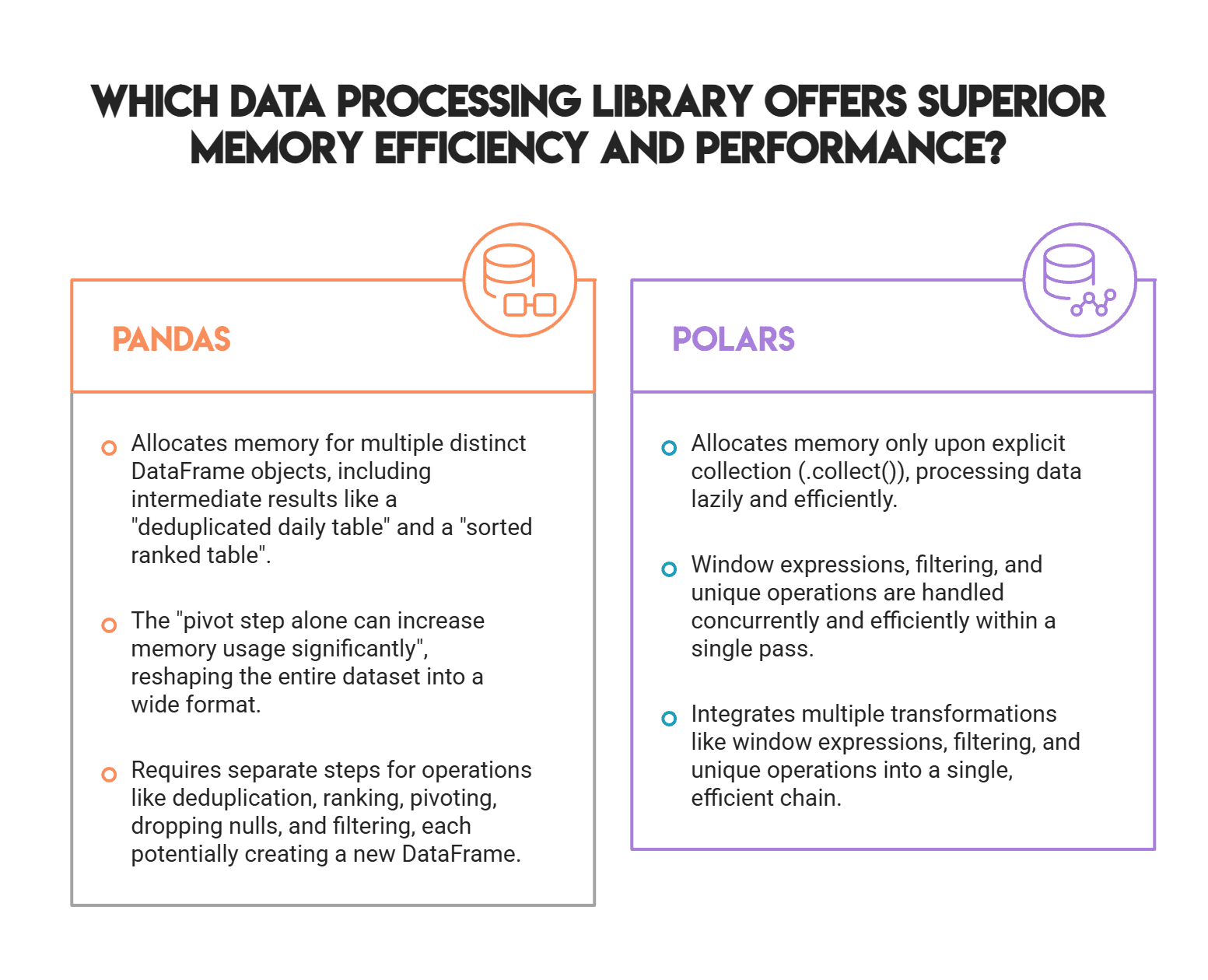
Pandas ソリューションにおける DataFrame の別個の割り当て数に注目してください:重複削除された日次テーブル、ソート済みランク付けテーブル、ピボットされたフレーム、dropna 結果、そしてフィルタリング後の出力です。これらはそれぞれが新しいメモリブロックへデータをコピーする 5 つの独立したオブジェクトで構成されています。大規模なトランザクションテーブルの場合、ピボットステップだけでメモリの使用量が大幅に増加し得ます。これは、データセット全体をワイド形式へと再整形するためです。
Polars の遅延実行チェーンは、.collect() を呼び出すまでメモリを一切割り当てません。.over("user_id") ウィンドウ式は各ユーザーの最初の購入日を 1 パスで計算し、.filter() は同じステップですぐに適用され、.unique() は CPU コア間で並列実行されます。ピボット操作も、中間のソート済みコピーも、日付の変換ステップも不要です。Polars は式エンジン内で日付演算をネイティブに処理します。このアプローチは、中規模程度のデータセットでもメモリ消費が少なく、高速に動作します。
以下にコード出力のプレビューを示します:
user_id
100
103
105
...
143
# expanding().mean() と cum_mean() の比較:月次売上移動平均
この質問 では、2022 年を通じた月次書籍売上の累積平均を算出するよう求められています。この平均は毎月、それまでのすべての月のデータを用いて更新されます。例えば、2 月は 1 月と 2 月の平均、3 月は 1 月から 3 月までの平均となり、以下同様に続きます。出力には、月次、その月の売上合計、そして小数点以下を四捨五入した累積平均を含める必要があります。
// データビュー
amazon_books テーブルは、各書籍と単価が 1 行ずつ格納されています。book_orders テーブルは、各注文が 1 行ずつ格納され、書籍 ID を数量と注文日に関連付けます。以下にテーブルのプレビューを示します:
book_id
book_title
unit_price
B001
The Hunger Games
25
B002
The Outsiders
50
B003
To Kill a Mockingbird
100
...
...
...
B020
The Pillars of the Earth
60
book_orders テーブルには、各注文 ID を注文日付、書籍 ID、および発注数量と関連付ける行が 1 つずつ含まれています:
order_id
order_date
book_id
quantity
1001
2022-01-10
B001
1
1002
2022-01-10
B009
1
1003
2022-01-15
B012
2
...
...
...
...
1084
2023-02-01
B009
1
粒度**(出力行 1 つが意味するもの): 2022 年の 1 ヶ月分であり、その月の売上合計と、その月を含むまでの全月の売上の累積平均値です。
// Trade-Offs
Pandas を使用する場合、.expanding().mean() クラウスは便利ですが、内部では成長するウィンドウのスライスに対して Python レベルのループで動作します。12 行分の月次集計であればこのコストは無視できるほど小さいものです。しかし、大規模な日次または時間別のデータ(例えば、3 年分の時間別取引など)の場合、各拡大ウィンドウスライスが追加するオーバーヘッドは行ごとに蓄積され、増幅されます。
Polars の cum_mean() は Rust で単一のパスを実行するため、スケールにおいては本質的に高速です。ただし、一つ注意が必要です。この質問では四捨五入して最も近い整数に丸めることが求められており、Pandas はデフォルトで銀行家流の丸め(半端を偶数へ丸める)を使用します。Polars の解決策では、NumPy の cumsum を使用し、明示的に floor(x + 0.5) という式を適用して、切り上げ型の丸め動作を強制しています。期待される出力と正確に一致させる必要がある場合、どちらのライブラリにも組み込まれている丸め処理よりも、NumPy メソッドの方が信頼性が高いです。
// Solutions
1. Pandas による解決策
書籍と注文を結合し、2022 年に絞り込み、月ごとの売上を集計して .expanding().mean() を適用し、累積平均を計算します。
import pandas as pd
import numpy as np
import datetime as dt
merged = pd.merge(book_orders, amazon_books, on="book_id", how="inner")
merged["order_date"] = pd.to_datetime(merged["order_date"])
merged["order_month"] = merged["order_date"].dt.month
merged["year"] = merged["order_date"].dt.year
merged["sales"] = merged["unit_price"] * merged["quantity"]
merged = merged.loc[(merged["year"] == 2022), :]
result = (
merged.groupby("order_month")["sales"]
.sum()
.to_frame("monthly_sales")
.sort_values(by="order_month")
.reset_index()
)
result["rolling_average"] = result["monthly_sales"].expanding().mean().round(0)
result
2. Polars: 遅延実行パイプラインの構築と収集
2 つのテーブルを遅延実行チェーン内で結合し、売上を単価×数量として計算し、2022 年に絞り込み、月ごとに集計した上で、NumPy のローリング処理の前に .collect() を呼び出して eager モードに切り替えます。
import polars as pl
import numpy as np
ステップ 1:月次売上(LazyFrame)の準備
monthly_sales_lazy = (
book_orders.lazy()
.join(amazon_books.lazy(), on="book_id", how="inner")
.with_columns([
(pl.col("unit_price") * pl.col("quantity")).alias("sales"),
pl.col("order_date").cast(pl.Datetime),
pl.col("order_date").dt.year().alias("year"),
pl.col("order_date").dt.month().alias("order_month")
])
.filter(pl.col("year") == 2022)
.group_by("order_month")
.agg(pl.col("sales").sum().alias("monthly_sales"))
.sort("order_month")
)
ステップ 2:ローリング計算のためにイーグルモード(Eager Mode)に切り替え
monthly_sales = monthly_sales_lazy.collect()
3. ローリング平均の計算と最終処理
月次売上を NumPy アレイとして扱い、半端切り上げ(round-half-up)による丸め処理を適用し、その結果を Polars DataFrame に戻して出力列を選択します。
ステップ 3:半値切り上げを用いたローリング平均の計算
sales_np = monthly_sales["monthly_sales"].to_numpy()
cumsum = np.cumsum(sales_np)
rolling_avg = np.floor(cumsum / np.arange(1, len(cumsum)+1) + 0.5).astype(int)
ステップ 4:Polars DataFrame に戻す
monthly_sales = monthly_sales.with_columns([
pl.Series("rolling_average", rolling_avg)
])
ステップ 5:正しい列名を持つ最終結果
result = monthly_sales.select(["order_month", "monthly_sales", "rolling_average"])
// パフォーマンス比較
**

この質問には、パフォーマンスに最も大きな影響を与える 2 つの操作があります。それは結合(join)と累積ウィンドウです。Pandas では、pd.merge はまず両方のテーブルからすべての行を結合し、その後で 2022 年を対象にフィルタリングします。つまり、対象期間外の行が破棄される前に、毎年分の注文データすべてが処理されます。一方、Polars は遅延クエリプラン(lazy query plan)を構築し、結合実行の前に filter(year == 2022) の条件をプッシュします。これにより、最初からより小さなデータセットで結合が行われます。この述語プッシュダウン(predicate pushdown)は、追加の記述なしに自動的に発生します。
最も顕著な違いは、ローリング平均の差です。Pandas の .expanding().mean() はウィンドウを 1 行ずつ拡大し、各セグメントで C 言語への呼び出しを行いつつ、Python ループによって制御されます。一方、Polars の cum_mean() は、Python のオーバーヘッドなしに Rust ループで列全体を一度に計算します。月次データではこの差が感知できない場合もありますが、3 年分の日次データ(約 1,000 行)で同じクエリを実行すると、Polars バージョンはマイクロ秒で完了するのに対し、Pandas は拡大ウィンドウによる測定可能なレイテンシを示します。
以下にコード出力のプレビューを示します:
order_month
sales
rolling_average
1
145
145
2
250
198
3
315
237
...
...
...
12
710
402
# 結論
上記の 3 つの問題すべてにおいて、Polars の解決策は同じパターンに従っています。すなわち、遅延クエリプランを構築し、可能な限り多くの計算をオプティマイザに押し込み、具体的な結果が必要になったときにのみ .collect() を呼び出すことです。
アナリストの多くが長年培ってきた Pandas の習慣に慣れ親しんでいる場合、構文にはいくつかの調整が必要ですが、操作内容は非常に近接しています。.groupby() は .group_by() に、.rename() は columns= キーワードではなく通常の辞書を受け取り、ランキング機能はソート後に .with_row_count() を実行することで実現されます。
真の違いが顕著になるのは大規模データ処理の場面です。小規模なデータセットを扱う場合、両ライブラリとも十分な速度で結果を返すため、その差は目立ちません。しかし、行数が数百万に達すると、Polars の Rust レベルでの並列処理と単一パスアルゴリズムにより、圧倒的なパフォーマンスの向上が見られます。Pandas でパフォーマンスの問題に直面している場合、これら 3 つの課題は移行のための優れた出発点となります。
Nate Rosidi はデータサイエンティストであり、製品戦略にも携わっています。また、分析を教える非常勤講師でもあり、トップ企業からの実際の面接質問を通じてデータサイエンティストの準備をサポートするプラットフォーム「StrataScratch」の創設者です。Nate はキャリア市場における最新動向について執筆し、面接に関するアドバイスを提供し、データサイエンスプロジェクトを紹介し、SQL 関連のあらゆるトピックをカバーしています。
原文を表示

**
# Introduction
Over the last decade, Pandas** has been the foundation for data work in Python. For datasets that fit in memory, it is fast and familiar enough that switching libraries rarely crosses any programmer's mind.
However, once you start working with millions of rows, the flaws start to appear: groupby operations that take several seconds, intermediate copies that consume RAM, and window functions that run as Python-level loops rather than vectorized C or Rust code.
Polars is a DataFrame library built in Rust on top of Apache Arrow. It was designed with parallelism and lazy evaluation as first-class features. Pandas executes each operation upfront and in sequence, whereas Polars can build up a query plan and optimize it prior to executing, with most operations executing concurrently across all available CPU cores automatically.
In this article, we explore three real data problems using real questions from the StrataScratch coding platform. For each problem, we compare both libraries' solutions and point out where the performance difference matters most.
**
# Using rank() vs. with_row_count(): Activity Rank
In this question, the goal is to find the email activity rank for each user based on the total number of emails sent. The user with the most emails gets rank 1. Results must be sorted by total emails in descending order, using alphabetical order as a tiebreaker, and each rank must be distinct, even if two users have the same email count.
// Data View
The google_gmail_emails table stores one row per email sent, with a sender ID (from_user), recipient ID (to_user), and the day the email was sent. Here is a preview of the table:
id
from_user
to_user
day
0
6edf0be4b2267df1fa
75d295377a46f83236
10
1
6edf0be4b2267df1fa
32ded68d89443e808
6
2
6edf0be4b2267df1fa
55e60cfcc9dc49c17e
10
3
6edf0be4b2267df1fa
e0e0defbb9ec47f6f7
6
4
...
...
...
314
e6088004caf0c8cc51
e6088004caf0c8cc51
5
Grain** (what one output row means): one user, with their total email count and unique activity rank.
// Common Mistake
The question asks for a unique rank even when two users have the same email count. A common mistake is to use the rank(method='dense') method in Pandas, which assigns the same rank to tied users. The correct method is 'first', which breaks ties by position in the sorted frame. Since we sort alphabetically by user_id before ranking, the resulting ranks are unique and deterministic.
The Polars optimal solution avoids the rank function entirely. After sorting by ["total_emails", "user_id"] in descending and ascending order, respectively, the .with_row_count("activity_rank", offset=1) clause assigns sequential integers starting from 1. No tie-breaking logic is needed because the sort already handled it.
// Solutions
1. Pandas Solution
We rename from_user to user_id, group by user, count emails, compute the first rank, and sort by email count in descending order, with alphabetical tie-breaking.
import pandas as pd
import numpy as np
google_gmail_emails = google_gmail_emails.rename(columns={"from_user": "user_id"})
result = google_gmail_emails.groupby(
['user_id']).size().to_frame('total_emails').reset_index()
result['activity_rank'] = result['total_emails'].rank(method='first', ascending=False)
result = result.sort_values(by=['total_emails', 'user_id'], ascending=[False, True])2. Polars Solution
We use a lazy chain that renames, groups, sorts, and assigns row numbers in a single pass. Calling .collect() at the end materializes the result.
import polars as pl
google_gmail_emails = google_gmail_emails.rename({"from_user": "user_id"})
result = (
google_gmail_emails.lazy()
.group_by("user_id")
.agg(total_emails = pl.count())
.sort(
by=["total_emails", "user_id"],
descending=[True, False]
)
.with_row_count("activity_rank", offset=1)
.select([
pl.col("user_id"),
"total_emails",
"activity_rank"
])
.collect()
)// Performance Comparison
**
The Pandas solution iterates over the data twice after grouping: once to compute sizes and once to assign ranks. Internally, rank(method='first') allocates a rank array, resolves ties via argsort, and writes back — which is considerably more expensive than it looks for a single column. The Polars group_by function divides the workload across all available CPU cores, resulting in significantly faster aggregation for large tables. And since the .with_row_count() clause is a single O(n) sequential pass after sorting, it replaces the rank function with the cheapest possible operation. On a table containing millions of email records, the use of parallel aggregation without a rank function can result in a 5–10x improvement in wall-clock time compared to the Pandas approach.
Here is the code output preview:
user_id
total_emails
activity_rank
32ded68d89443e808
19
1
ef5fe98c6b9f313075
19
2
5b8754928306a18b68
18
3
55e60cfcc9dc49c17e
16
4
91f59516cb9dee1e88
16
5
...
...
...
e6088004caf0c8cc51
6
25
# Using cumcount() + pivot() vs. over(): Finding User Purchases
In this question, we're asked to identify returning active users — specifically, those who made a second purchase within 1 and 7 days after their first. Purchases made on the same day should not be included. The result is simply a list of qualifying user_id values.
// Data View
The amazon_transactions table has one row per purchase, with user_id, item, created_at date, and revenue.
Here is a preview of the table:
id
user_id
item
created_at
revenue
1
109
milk
2020-03-03
123
2
139
biscuit
2020-03-18
421
3
120
milk
2020-03-18
176
...
...
...
...
...
100
117
bread
2020-03-10
209
Grain** (what one output row means): one user ID that made a qualifying return purchase within 7 days of their first.
// Edge Case
Same-day purchases should be ignored, meaning the gap between first and second purchase must exceed 0 days and be at most 7 days. A customer who buys twice on the same day does not qualify.
// Solutions
Both solutions find each user's earliest purchase date and then filter for subsequent purchases within the 1- to 7-day timeframe. One thing to watch: if created_at has timestamps instead of plain dates, you need to truncate to the date before comparing. Otherwise, two purchases made at different times on the same day would incorrectly pass the strict inequality.
1. Pandas Solution
In Pandas, the solution involves isolating unique purchase dates per user, ranking them with cumcount(), pivoting to get first and second dates side by side, and computing the day difference.
import pandas as pd
amazon_transactions["purchase_date"] = pd.to_datetime(amazon_transactions["created_at"]).dt.date
daily = amazon_transactions[["user_id", "purchase_date"]].drop_duplicates()
ranked = daily.sort_values(["user_id", "purchase_date"])
ranked["rn"] = ranked.groupby("user_id").cumcount() + 1
first_two = (ranked[ranked["rn"] <= 2]
.pivot(index="user_id", columns="rn", values="purchase_date")
.reset_index()
.rename(columns={1: "first_date", 2: "second_date"}))
first_two = first_two.dropna(subset=["second_date"])
first_two["diff"] = (pd.to_datetime(first_two["second_date"]) - pd.to_datetime(first_two["first_date"])).dt.days
result = first_two[(first_two["diff"] >= 1) & (first_two["diff"] <= 7)][["user_id"]]2. Polars Solution
The Polars solution involves computing the first purchase date per user as a window expression with .over("user_id"), filtering to purchases that fit the time window, and returning a deduplicated user_id list.
import polars as pl
# returning active users: 2nd purchase 1–7 days after the first (ignore same-day)
returning_users = (
    amazon_transactions
    .lazy()
    # first purchase date per user (window so we avoid .groupby on LazyFrame)
    .with_columns(
        pl.col("created_at").min().over("user_id").alias("first_purchase_date")
    )
    # keep transactions strictly 1-7 days after that first purchase
    .filter(
        (pl.col("created_at") > pl.col("first_purchase_date")) &
        (pl.col("created_at") <= pl.col("first_purchase_date") + pl.duration(days=7))
    )
    # distinct user list
    .select("user_id")
    .unique()
    .sort("user_id", descending=[False])
)
// Performance Comparison
**
Notice the number of distinct DataFrame allocations in the Pandas solution: the deduplicated daily table, the sorted ranked table, the pivoted frame, the dropna result, and the filtered output. These consist of five separate objects, each of which copies data into a new memory block. On a large transactions table, the pivot step alone can significantly increase memory usage, as it reshapes the entire dataset into a wide format.
The Polars lazy chain does not allocate any memory until .collect(). The .over("user_id") window expression computes each user's earliest purchase date in one pass, the .filter() applies immediately in the same step, and .unique() runs concurrently across CPU cores. There is no pivot, no intermediate sorted copy, and no separate date-casting step — Polars handles date arithmetic natively inside the expression engine. This approach consumes less memory and runs faster, even on moderately sized datasets.
Here is the code output preview:
user_id
100
103
105
...
143
# Using expanding().mean() vs. cum_mean(): Monthly Sales Rolling Average
In this question, we're asked to determine a cumulative average for monthly book sales throughout 2022. The average grows each month using all preceding months: February averages January and February, March averages all three, and so on. The output should include the month, that month's total sales, and the cumulative average rounded to the nearest whole number.
// Data View
The amazon_books table has one row per book and its unit price. The book_orders table has one row per order, linking a book ID to a quantity and an order date. Here is a preview of the table:
book_id
book_title
unit_price
B001
The Hunger Games
25
B002
The Outsiders
50
B003
To Kill a Mockingbird
100
...
...
...
B020
The Pillars of the Earth
60
The book_orders table has one row per book order, linking each order ID to an order date, book ID, and the quantity ordered:
order_id
order_date
book_id
quantity
1001
2022-01-10
B001
1
1002
2022-01-10
B009
1
1003
2022-01-15
B012
2
...
...
...
...
1084
2023-02-01
B009
1
Grain** (what one output row means): one month in 2022, with total sales for that month and a cumulative average of all monthly sales up to and including that month.
// Trade-Offs
Using Pandas, the .expanding().mean() clause is convenient, but operates internally with a Python-level loop over growing window slices. For a 12-row monthly summary, this cost is negligible. For daily or hourly data at scale (say, three years of hourly transactions), each expanding window slice adds overhead that compounds row by row.
Polars' cum_mean() runs a single pass in Rust and is inherently faster at scale. There is one catch: the question requires rounding to the nearest whole number, and Pandas uses banker's rounding (round half to even) by default. The Polars solution uses NumPy's cumsum with an explicit floor(x + 0.5) formula to enforce round-half-up behavior. If you need an exact match to the expected output, the NumPy method is more reliable than the built-in rounding in either library.
// Solutions
1. Pandas Solution
We merge books with orders, filter to 2022, aggregate monthly sales, and apply .expanding().mean() to compute the cumulative average.
import pandas as pd
import numpy as np
import datetime as dt
merged = pd.merge(book_orders, amazon_books, on="book_id", how="inner")
merged["order_date"] = pd.to_datetime(merged["order_date"])
merged["order_month"] = merged["order_date"].dt.month
merged["year"] = merged["order_date"].dt.year
merged["sales"] = merged["unit_price"] * merged["quantity"]
merged = merged.loc[(merged["year"] == 2022), :]
result = (
    merged.groupby("order_month")["sales"]
    .sum()
    .to_frame("monthly_sales")
    .sort_values(by="order_month")
    .reset_index()
)
result["rolling_average"] = result["monthly_sales"].expanding().mean().round(0)
result
2. Polars: Building the Lazy Pipeline and Collecting
We join the two tables inside a lazy chain, compute sales as unit_price * quantity, filter to 2022, aggregate by month, and call .collect() to switch to eager mode before the NumPy rolling step.
import polars as pl
import numpy as np
# Step 1: Prepare monthly sales (LazyFrame)
monthly_sales_lazy = (
    book_orders.lazy()
    .join(amazon_books.lazy(), on="book_id", how="inner")
    .with_columns([
        (pl.col("unit_price") * pl.col("quantity")).alias("sales"),
        pl.col("order_date").cast(pl.Datetime),
        pl.col("order_date").dt.year().alias("year"),
        pl.col("order_date").dt.month().alias("order_month")
    ])
    .filter(pl.col("year") == 2022)
    .group_by("order_month")
    .agg(pl.col("sales").sum().alias("monthly_sales"))
    .sort("order_month")
)
# Step 2: Switch to eager mode for rolling computation
monthly_sales = monthly_sales_lazy.collect()
3. Computing the Rolling Average and Finalizing
With the monthly sales as a NumPy array, we apply round-half-up rounding, add the result back to the Polars DataFrame, and select the output columns.
# Step 3: Rolling average with round-half-up
sales_np = monthly_sales["monthly_sales"].to_numpy()
cumsum = np.cumsum(sales_np)
rolling_avg = np.floor(cumsum / np.arange(1, len(cumsum)+1) + 0.5).astype(int)
# Step 4: Add back to Polars DataFrame
monthly_sales = monthly_sales.with_columns([
    pl.Series("rolling_average", rolling_avg)
])
# Step 5: Final result with correct column names
result = monthly_sales.select(["order_month", "monthly_sales", "rolling_average"])
// Performance Comparison
**
This question has two operations that affect performance the most: the join and the cumulative window. In Pandas, pd.merge joins all rows from both tables before filtering for 2022. This means that every year's worth of orders is processed before rows outside the target period are discarded. Polars builds a lazy query plan and pushes the filter(year == 2022) condition before the join executes, so it joins a smaller dataset from the start. That predicate pushdown happens automatically, with no extra writing required.
The most noticeable difference is the rolling average gap. Pandas' .expanding().mean() grows its window one row at a time, calling into C for each segment while remaining controlled by a Python loop. Polars' cum_mean() computes the whole column in a single Rust loop with no Python overhead. While the difference may be imperceptible with monthly data, if you run this same query on daily data for three years (roughly 1,000 rows), the Polars version completes in microseconds while Pandas shows measurable latency due to the expanding window.
Here is the code output preview:
order_month
sales
rolling_average
1
145
145
2
250
198
3
315
237
...
...
...
12
710
402
# Conclusion
Across all three problems, the Polars solutions follow the same pattern: build a lazy query plan, push as much computation as possible into the optimizer, and call .collect() only when you need a concrete result.
The syntax takes some adjustment if you, like most analysts, have years of Pandas habits, but the operations align closely. .groupby() becomes .group_by(), .rename() takes a plain dict instead of a columns= keyword, and ranking becomes a sort followed by .with_row_count().
The true difference shows at scale. When dealing with small datasets, both libraries return results fast enough that the difference is not noticeable. As row counts reach the millions, Polars' Rust-level parallelism and single-pass algorithms significantly outperform. If you're encountering performance issues with Pandas, these three challenges are a great starting point for migration.
Nate Rosidi** is a data scientist and in product strategy. He's also an adjunct professor teaching analytics, and is the founder of StrataScratch, a platform helping data scientists prepare for their interviews with real interview questions from top companies. Nate writes on the latest trends in the career market, gives interview advice, shares data science projects, and covers everything SQL.
関連記事
今日のまとめ
AI日報で今日の重要ニュースをまとめ読み