Pandas でループを書かない：試すべき 7 つの高速代替案

![image](https://www.kdnuggets.com/wp-content/uploads/kdn-pandas-alts-to-loops.png)** ## # イントロダクション 行ごとの反復処理は、[pandas](https://pandas.pydata.org/) コードにおける最も一般的なパフォーマンスのボトルネックの一つです。小規模なデータセットでは目立たないこともありますが、[大規模データの処理](https://www.kdnuggets.com/how-to-handle-large-datasets-in-python-even-if-youre-a-beginner)においては大きな影響を及ぼします。 pandas は [NumPy](https://numpy.org/) を基盤として構築されており、コンパイルされた C コードを使用して配列全体に対して一度に演算を実行します。Python で行をループ処理することはこれを完全に迂回し、すべての操作を Python インタープリタに戻すことになります — 1 行ずつです。 この記事では、pandas におけるループの代替手段として 7 つの方法を取り上げます。それぞれが異なる種類の変換に適しています。最後には、問題の形状に応じてどのツールを使うべきかという明確な思考マップを得られるでしょう。 [Colab ノートブックは GitHub で入手できます](https://github.com/balapriyac/data-science-tutorials/tree/main/pandas/what-to-use-instead-of-looping)。 ## # サンプルデータのセットアップ 本記事全体を通じて、現実的な e コマース注文データセットを使用します： import pandas as pd import numpy as np np.random.seed(42) n = 100_000 categories = ['Electronics', 'Clothing', 'Home & Kitchen', 'Sports', 'Books'] regions = ['North', 'South', 'East', 'West'] df = pd.DataFrame({ 'order_id': range(1, n + 1), 'customer_age': np.random.randint(18, 70, n), 'product_category': np.random.choice(categories, n), 'region': np.random.choice(regions, n), 'price': np.round(np.random.uniform(5.0, 500.0, n), 2), 'quantity': np.random.randint(1, 10, n), 'days_to_ship': np.random.randint(1, 14, n), }) display(df.head()) Output: ![image](https://www.kdnuggets.com/wp-content/uploads/kdn-pd-loop-alt-create-df.png) 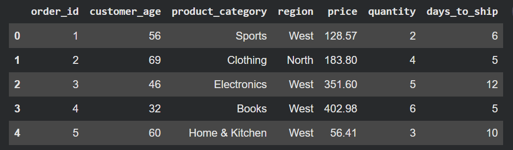これで、作業に使える 10 万件の行を持つデータセットが完成しました。 ## # 1. 算術演算にはベクトル化演算を使用する 列に対する任意の算術演算や比較においては、[ベクトル化演算 (Vectorized Operations)](https://www.pythonlikeyoumeanit.com/Module3_IntroducingNumpy/VectorizedOperations.html) がまず最初に思い浮かぶべき手法です。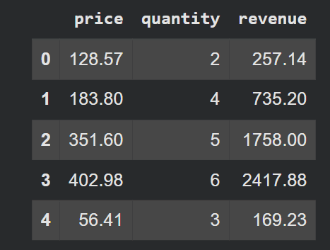 **私たちが行いたいこと**: 注文ごとの総売上高を計算する。 df['revenue'] = df['price'] * df['quantity'] display(df[['price', 'quantity', 'revenue']].head()) Output: ** ![image](https://www.kdnuggets.com/wp-content/uploads/kdn-pd-loop-alt-1.png) ## # 2. 条件付きロジックには関数の適用を使用する 単純な算術演算では表現できない論理を含む変換を行う場合、[.apply()](https://pandas.pydata.org/docs/reference/api/pandas.DataFrame.apply.html) を使用すると、列または行に対して関数を渡すことができます。 **私たちが行いたいこと**: 配送までの日数に基づいて配送優先度のラベルを割り当てる。 def shipping_label(days): if days <= 2: return 'Express' elif days <= 5: return 'Standard' else: return 'Economy' df['shipping_tier'] = df['days_to_ship'].apply(shipping_label) display(df[['days_to_ship', 'shipping_tier']].head()) Output: ![image](https://www.kdnuggets.com/wp-content/uploads/kdn-pd-loop-alt-2.png) . 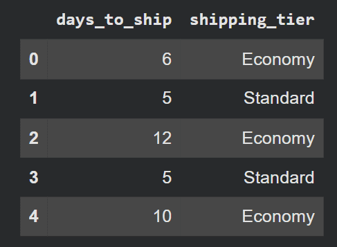apply() を使用すると、コードが清潔で読みやすく、ループよりもはるかにデバッグしやすいです。ロジックが条件分岐であり、np.where() や np.select() がネストしすぎてしまう場合にこれを使用してください。 ## # 3. 二値条件には np.where() を使用する ** 二値条件（真の場合と偽の場合でそれぞれ異なる結果を返す場合）があるときは、[np.where()](https://numpy.org/devdocs/reference/generated/numpy.where.html) が清潔かつ高速な選択肢です。 ** 実行したいこと**: 顧客がシニア割引の対象となる注文にフラグを立てることです。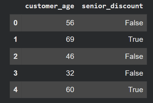 df['senior_discount'] = np.where(df['customer_age'] >= 60, True, False) display(df[['customer_age', 'senior_discount']].head()) Output: ![image](https://www.kdnuggets.com/wp-content/uploads/kdn-pd-loop-alt-3.png) np.where() は完全にベクトル化されており、単純な真偽条件においては .apply() よりも大幅に高速です。これはベクトル化された三項演算子と考えることができます。 ## # 4. np.select() を使用して複数の条件から選択する ** 2 つ以上の条件がある場合、[np.select()](https://numpy.org/doc/stable/reference/generated/numpy.select.html) を使用すると、ネストされた if/elif 連鎖を一切必要とせずに、条件のリストと対応する値を定義できます。 私たちが行いたいこと**: リージョンベースの税率を割り当てることです。 conditions = [ df['region'] == 'North', df['region'] == 'South', df['region'] == 'East', df['region'] == 'West', ] tax_rates = [0.08, 0.06, 0.07, 0.09] df['tax_rate'] = np.select(conditions, tax_rates, default=0.07) df['tax_amount'] = df['price'] * df['tax_rate'] display(df[['region', 'price', 'tax_rate', 'tax_amount']].head()) 出力: ![image](https://www.kdnuggets.com/wp-content/uploads/kdn-pd-loop-alt-4.png) 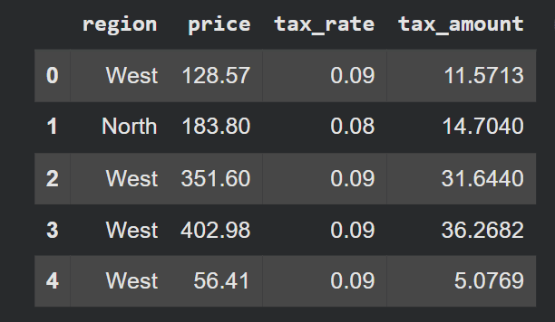np.select() は条件を順番に評価し、最初の一致するものを選択します。default パラメータは一致しないものを処理するため、安全網として有用です。 ## # 5. ディクショナリ参照による値のマッピング ** カラム内の値を変換する場合 — カテゴリ名を数値コードにマッピングしたり、キーをラベルに置き換えたりする場合など — [.map()](https://pandas.pydata.org/docs/reference/api/pandas.DataFrame.map.html) をディクショナリと併用すると、すっきりとして高速です。 私たちが行いたいこと**: 製品カテゴリを内部部門コードにマッピングすることです。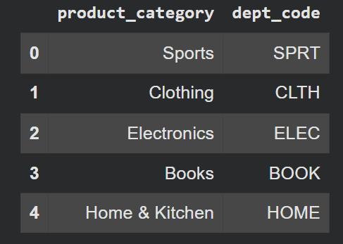 category_codes = { 'Electronics': 'ELEC', 'Clothing': 'CLTH', 'Home & Kitchen': 'HOME', 'Sports': 'SPRT', 'Books': 'BOOK', } df['dept_code'] = df['product_category'].map(category_codes) display(df[['product_category', 'dept_code']].head()) 出力: ![image](https://www.kdnuggets.com/wp-content/uploads/kdn-pd-loop-alt-5.png) .map() は照合テーブルとして機能します。これは pandas において最も過小評価されているツールの一つです—私たちは .map(dict) が同じことをより高速に実行するにもかかわらず、.apply(lambda x: dict[x]) を使用しがちです。 ## # 6. .str アクセサによる文字列操作 ** [文字列操作](https://www.kdnuggets.com/15-useful-python-one-liners-string-manipulation) は、人々が最も頻繁にループや .apply() に頼ってしまう分野です。[.str アクセサ](https://pandas.pydata.org/docs/user_guide/text.html#string-methods) を使用すれば、これらいずれも使わずに、列全体に対して文字列操作を実行できます。 私たちがやりたいこと**: product_category 列から最初の単語を抽出し、それを小文字に変換することです。 df['category_slug'] = df['product_category'].str.split().str[0].str.lower() display(df[['product_category', 'category_slug']].head()) 出力: ## # 7. .groupby() を用いたグループ集約 ** 一般的なループのパターンは、データのサブセットを反復処理してグループレベルの統計量を計算することです。[.groupby()](https://pandas.pydata.org/docs/reference/api/pandas.DataFrame.groupby.html) はこれをネイティブで処理します。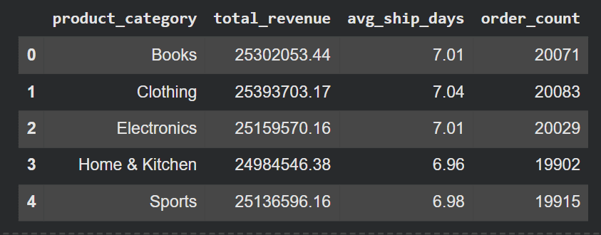 私たちがやりたいこと**: 製品カテゴリごとの総売上高と出荷までの平均日数を計算することです。 summary = ( df.groupby('product_category') .agg( total_revenue=('revenue', 'sum'), avg_ship_days=('days_to_ship', 'mean'), order_count=('order_id', 'count') ) .round(2) .reset_index() ) summary ** ![image](https://www.kdnuggets.com/wp-content/uploads/kdn-pd-loop-alt-7.png) ## # 適切なツールの選択 ループで記述するほとんどの変換は、以下のいずれかのパターンにきれいに収まります: 操作 / メソッド | 使用例 / 説明 ---|--- 列の算術演算 | DataFrame の列に対して、加算、減算、乗算、除算などのベクトル化された数学演算を直接実行します。 ベクトル化演算 (*, + など) | 明示的なループなしで、効率的に全列に要素ごとの演算を適用します。 単純な真偽条件 | ブール条件を評価してフィルタリングしたり、条件付きカラムを作成したりします。 np.where() | 配列や DataFrame の列に対して、条件分岐 (if-else) ロジックをベクトル化された方法で適用します。 複数の条件と複数の結果 | 複数のルールと出力を持つ複雑な条件ロジックを処理します。 np.select() | 複数の条件に基づいて値を選択し、対応する出力を返します。 ルックアップによる値の置換 | 変換用辞書を使用して値を置き換え、高速な変換を実現します。 .map(dict) | シリーズ内の値を辞書または関数でマッピングして置換します。 .apply() | カスタム関数を行単位または列単位に適用し、柔軟な変換を行います。 文字列操作 .str アクセサーを使用してベクトル化された文字列操作を行い、テキストデータのクリーニングと変換を行ってください。 .groupby() + .agg() data をグループ化し、合計、平均、カウントなどの集計統計を計算します。 行ではなく列で考えるようになると、pandas API が単なる回避策というよりも、実際に意図された作業方法のように感じられるようになります。

Pandas でループを書かない：試すべき 7 つの高速代替案

背景や根拠まで確認しますか？

調べる

選ぶ

サイト