例題付きで解説するPandasのGroupBy機能
KDnuggets の記事は、Pandas の GroupBy 機能を用いた小売データ分析の実践的なチュートリアルを提供し、集計計算の効率的な実行方法を解説している。
キーポイント
GroupBy 機能の概要と利点
Pandas の GroupBy は、カテゴリ別にデータをグループ化して集計・要約する強力なツールであり、手動フィルタリングに代わり効率的な分析を可能にする。
サンプルデータの構築と前処理
注文 ID、地域、カテゴリー、販売担当者などの列を含む小売売上データセットを作成し、粗売上と純売上という新列を追加して分析準備を行う。
実践的な集計計算の例示
地域別総収益や製品カテゴリ別の平均注文金額など、具体的なビジネス質問に対する回答を GroupBy を用いて算出する手順が示されている。
サンプルデータの構築と計算
order_id, region, category などのカラムを持つ小売販売データセットを作成し、units と unit_price から gross_sales を、さらに discount を適用して net_sales を算出する新しい列を追加します。
基本の GroupBy 構文
グループ化したいカラム(例:region)を指定し、集計対象のカラム(例:net_sales)を選択した上で、sum() などの集計関数を適用するシンプルなパターンが最も一般的な使用法です。
地域別売上合計の算出
データセットを region でグループ化して各地域の net_sales の合計値を計算することで、North, South, West ごとに異なる総売上が即座に確認できます。
複数カラムによるグルーピング
複数のカラム(例:region と category)を指定してグループ化することで、異なる次元にわたる詳細なデータ分析が可能になります。
影響分析・編集コメントを表示
影響分析
この記事は AI モデル開発そのものへの直接的な革新をもたらすものではありませんが、データ分析基盤である Python/Pandas の活用スキル向上に寄与します。データサイエンティストやエンジニアにとって、大規模データを効率的に処理・解釈するための基礎的なベストプラクティスを提供しており、実務における生産性向上に直結する価値があります。
編集コメント
本記事は特定の AI 技術の進展を報じるものではなく、データ分析ツールの基礎的な使い方を解説する教育的コンテンツです。
 image**
# イントロダクション
Pandas は、データ分析のための最も人気のある Python ライブラリの一つです。構造化データのクリーニング、整形、集約、探索のためにシンプルなツールを提供します。Pandas の中でも特に有用な機能の一つが GroupBy** です。これは、1 つ以上のカテゴリに基づいて行をグループ化して回答が必要な質問に答えるのに役立ちます。
例えば、販売データを扱っている場合、地域ごとの総収益や製品カテゴリごとの平均注文額、各営業担当者が処理した注文数などを計算したいかもしれません。各カテゴリを手動で一つずつフィルタリングする代わりに、GroupBy を使用すれば、これらの計算をクリーンかつ効率的に行うことができます。
本チュートリアルでは、小さな販売データセットを用いた Pandas GroupBy の実用的な例を見ていきます。コーディング環境には Deepnote を使用しており、一部の出力はコードブロックの直下にノートブックのスクリーンショットとして表示されます。
# サンプルデータの作成
**
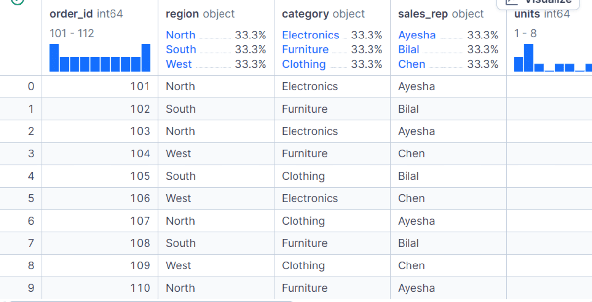
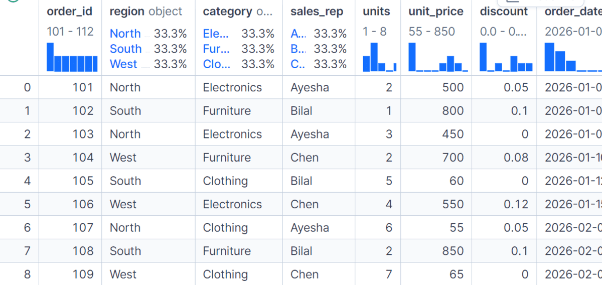
GroupBy を使用する前に、まず order_id、region(地域)、category(カテゴリ)、sales_rep(営業担当者)、units(数量)、unit_price(単価)、discount(割引)、order_date(注文日)などの列を持つ小売販売のサンプルデータセットを作成します。その後、辞書を変換して pandas DataFrame を作成し、gross_sales(総売上高)と net_sales(純売上高)という 2 つの新規列を追加します。
data = {
    "order_id": [101, 102, 103, 104, 105, 106, 107, 108, 109, 110, 111, 112],
    "region": ["North", "South", "North", "West", "South", "West", "North", "South", "West", "North", "South", "West"],
    "category": ["Electronics", "Furniture", "Electronics", "Furniture", "Clothing", "Electronics",
                 "Clothing", "Furniture", "Clothing", "Furniture", "Electronics", "Clothing"],
    "sales_rep": ["Ayesha", "Bilal", "Ayesha", "Chen", "Bilal", "Chen",
                  "Ayesha", "Bilal", "Chen", "Ayesha", "Bilal", "Chen"],
    "units": [2, 1, 3, 2, 5, 4, 6, 2, 7, 1, 2, 8],
    "unit_price": [500, 800, 450, 700, 60, 550, 55, 850, 65, 750, 520, 70],
    "discount": [0.05, 0.10, 0.00, 0.08, 0.00, 0.12, 0.05, 0.10, 0.00, 0.07, 0.03, 0.00],
    "order_date": pd.to_datetime([
        "2026-01-05", "2026-01-06", "2026-01-08", "2026-01-10",
        "2026-01-12", "2026-01-15", "2026-02-02", "2026-02-05",
        "2026-02-08", "2026-02-12", "2026-02-15", "2026-02-20"
    ])
}

df = pd.DataFrame(data)

df["gross_sales"] = df["units"] * df["unit_price"]
df["net_sales"] = df["gross_sales"] * (1 - df["discount"])

df
gross_sales(粗売上)列は、単価に販売数量を乗算することで計算され、net_sales(純売上)はその値から割引率を適用して調整したものです。これにより、すべての GroupBy 例で使用できるクリーンなデータセットが用意されます。
# 基本的な GroupBy 構文の使用
最も基本的な GroupBy 操作は、単純なパターンに従います:グループ化対象の列を選択し、値の列を選択し、集計関数を適用します。この例では、データを地域ごとにグループ化し、各地域の総ネット売上高を計算します。
df.groupby("region")["net_sales"].sum()
結果は、北、南、西がそれぞれ独自の合計売上値を持っていることを示しています。これは、データを要約する際の GroupBy の最も単純で一般的な使用例です。
region
North    3311.0
South    3558.8
West     4239.0
Name: net_sales, dtype: float64
# as_index=False を使用した GroupBy
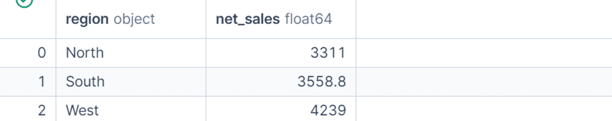
デフォルトでは、pandas は出力においてグループ化された列をインデックスとして使用します。これは場合によっては有用ですが、グループ化された列が通常の列のまま残る通常の DataFrame で作業する方が簡単なことがよくあります。そこで便利なのが as_index=False です。
df.groupby("region", as_index=False)["net_sales"].sum()
この例でも、地域ごとの総ネット売上高を計算しますが、結果はクリーンな DataFrame として返されるため、エクスポートや結合、レポートでの使用が容易になります。
# 1 つの列への複数の集計関数の適用
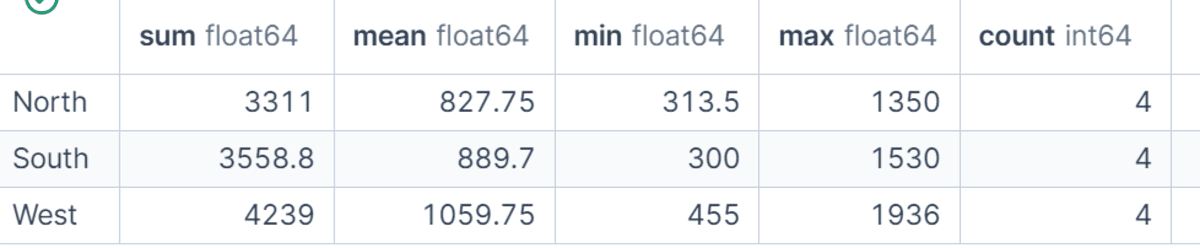
GroupBy は単一の計算に限定されません。agg() を使用して、同じ列に対して複数の集計関数を適用できます。
この例では、各地域のネット売上高について、合計、平均、最小値、最大値、および件数(count)を計算します。
これにより、地域別の売上パフォーマンスの簡易的な統計サマリーが得られ、総収益だけでなく、平均注文サイズや注文ボリュームも比較できるようになります。
df.groupby("region")["net_sales"].agg(["sum", "mean", "min", "max", "count"])
# 名前付き集約の使用
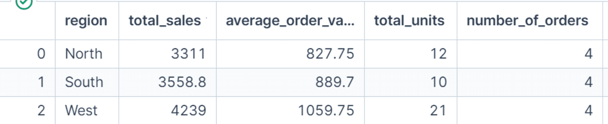
名前付き集約(Named Aggregations)を使用すると、GroupBy の出力がより読みやすく、扱いやすくなります。sum や mean といった汎用的な列名を返す代わりに、total_sales、average_order_value、total_units、number_of_orders といった独自の名称を定義できます。
これは、ダッシュボードやレポート、チュートリアル用の分析データを準備する際に特に役立ちます。出力の列名が各指標が何を表しているかを明確に説明するためです。
region_summary = (
    df.groupby("region", as_index=False)
      .agg(
          total_sales=("net_sales", "sum"),
          average_order_value=("net_sales", "mean"),
          total_units=("units", "sum"),
          number_of_orders=("order_id", "count")
      )
)

region_summary
# 複数の列によるグループ化
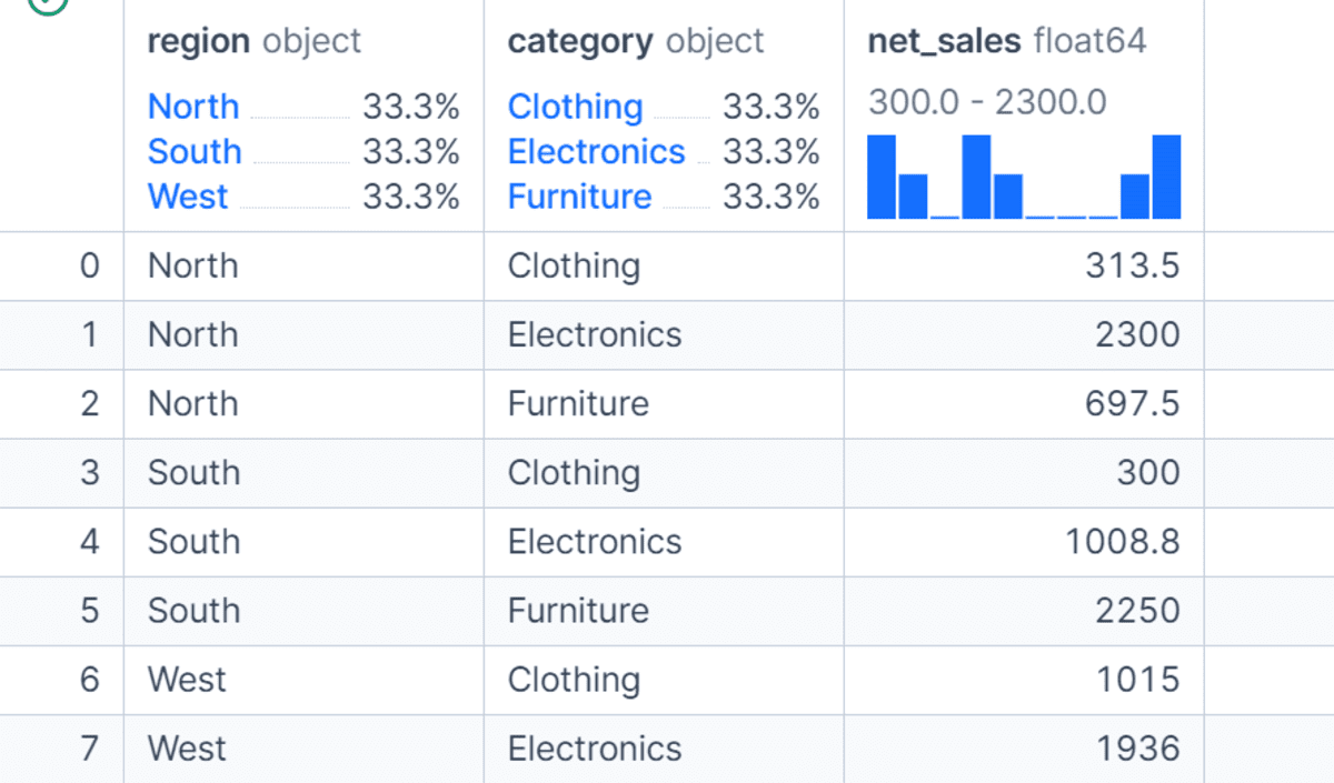
1 つ以上の列でデータをグループ化することも可能です。この例では、地域とカテゴリの両方でグループ化し、各地域内の各製品カテゴリごとの総純売上高を計算します。
これは、地域だけでグループ化する場合と比較して、データの詳細なビューを提供します。複数の列によるグループ化は、地域と製品、部署と従業員、月と顧客セグメントなど、異なる次元にわたってパフォーマンスを分析したい場合に有用です。
df.groupby(["region", "category"], as_index=False)["net_sales"].sum()
# グループ化結果のソート
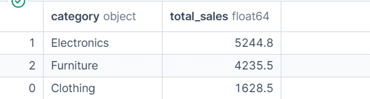
グループ化と集計の後、最高値または最低値を見つけるために結果をソートしたいことがよくあります。
この例では、製品カテゴリごとの総売上を計算し、結果を降順でソートします。
これにより、どのカテゴリが最も多くの収益を生んだかを簡単に特定できます。グループ化された結果のソートは、生データからの要約を実用的なインサイトに変換する際のシンプルかつ強力なステップです。
category_sales = (
    df.groupby("category", as_index=False)
      .agg(total_sales=("net_sales", "sum"))
      .sort_values("total_sales", ascending=False)
)

category_sales
# count と size の理解
Pandas には count() と size() の両方が用意されていますが、これらは完全に同じではありません。size() メソッドは、欠損値を含む行を含めて各グループの行数全体をカウントします。一方、count() メソッドは、選択された列内の非欠損値のみをカウントします。
この例では、意図的に sales_rep カラムに欠損値を追加しています。出力を見ると、size() は依然として各リージョンに対して 4 行をカウントしているのに対し、count() は sales_rep の値が一つ欠けているため North リージョンに対して 3 を返します。
import numpy as np

df_missing = df.copy()
df_missing.loc[2, "sales_rep"] = np.nan

print("Using size():")
display(df_missing.groupby("region").size())

print("Using count() on sales_rep:")
display(df_missing.groupby("region")["sales_rep"].count())
Output:
Using size():
region
North    4
South    4
West     4
dtype: int64

Using count() on sales_rep:
region
North    3
South    4
West     4
Name: sales_rep, dtype: int64
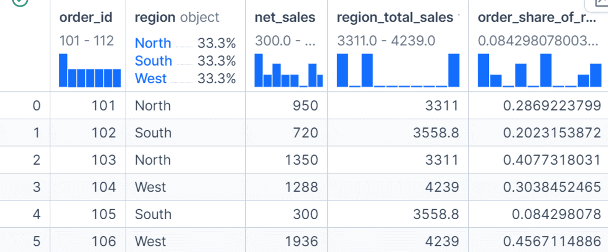
# Group レベルの特徴量計算のための transform() の使用
transform() メソッドは、グループレベルの値を計算して元の DataFrame に追加したい場合に便利です。
この例では、各リージョンの総売上を計算し、region_total_sales という新しいカラムに格納します。
次に、各注文が属するリージョンの総売上に占める割合を計算します。agg() がグループごとに 1 行にデータを縮約するのに対し、transform() は元の行と整合性のある値を返すため、特徴量エンジニアリングにおいて非常に有用です。
df["region_total_sales"] = df.groupby("region")["net_sales"].transform("sum")
df["order_share_of_region"] = df["net_sales"] / df["region_total_sales"]

df[["order_id", "region", "net_sales", "region_total_sales", "order_share_of_region"]]
# filter() を用いたグループのフィルタリング
filter() メソッドを使用すると、条件に基づいて特定のグループ全体を保持または削除できます。この例では、ネット販売額の合計が 3,000 より大きい地域のみを保持します。
各グループごとに要約行を 1 つ返すのではなく、filter() は条件を満たすグループから元の行をすべて返します。これは、パフォーマンスの低いグループを削除したり、特定のビジネスルールに合致するグループのみを残したい場合に役立ちます。
high_sales_regions = df.groupby("region").filter(lambda group: group["net_sales"].sum() > 3000)

high_sales_regions
# apply() を用いたカスタムロジックの適用
apply() メソッドは、各グループに対してカスタムのロジックを実行できるため、より柔軟性があります。
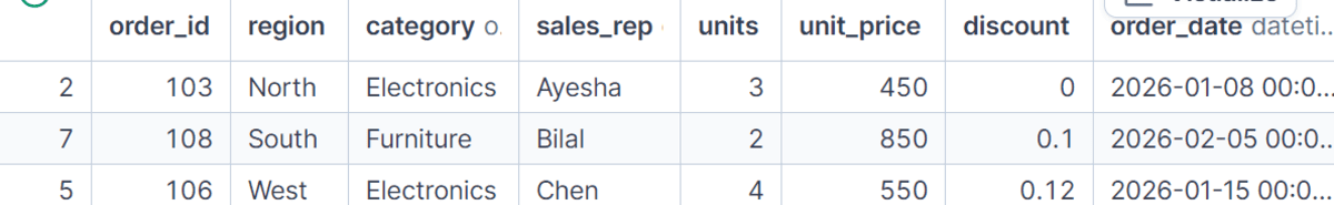
この例では、apply() と nlargest() を組み合わせて、各地域でネット販売額が最も高い上位 1 つの注文を見つけます。これは、組み込みの集計関数だけでは分析要件を満たせない場合に有用です。
ただし、apply() は sum(), mean(), agg(), transform() などの組み込みメソッドに比べて処理速度が遅くなる可能性があるため、カスタムなグループごとの操作が必要な場合のみ使用することが推奨されます。
top_order_by_region = (
    df.groupby("region", group_keys=False)
      .apply(lambda group: group.nlargest(1, "net_sales"))
)

top_order_by_region
# 日付によるグループ化
GroupBy は、時間ベースの分析にも非常に有用です。
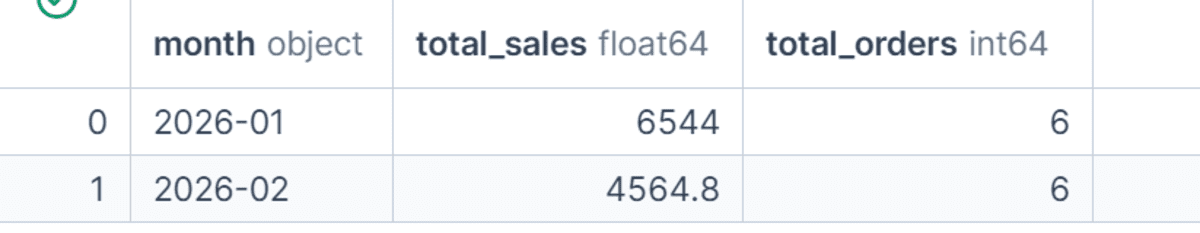
この例では、order_date カラムから月を抽出し、データを月ごとにグループ化します。その後、各月の売上合計と注文数を計算します。このアプローチは、月次売上や週ごとのユーザー活動、年間の収益成長など、時間の経過に伴う傾向を分析する際に役立ちます。
df["month"] = df["order_date"].dt.to_period("M").astype(str)

monthly_sales = (
    df.groupby("month", as_index=False)
      .agg(total_sales=("net_sales", "sum"), total_orders=("order_id", "count"))
)

monthly_sales
# pd.Grouper を用いた日付によるグループ化
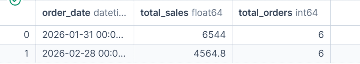
pd.Grouper は、別途月ごとのカラムを手動で作成することなく、時系列データをグループ化するよりクリーンな方法を提供します。
この例では、DataFrame を order_date によって月次頻度でグループ化し、売上合計と注文数を計算します。
これは、タイムスタンプを含む実世界のデータセットを扱い、日次、週次、月次、四半期、または年次でデータを要約したい場合に特に有用です。
monthly_sales_grouper = (
    df.groupby(pd.Grouper(key="order_date", freq="M"))
      .agg(total_sales=("net_sales", "sum"), total_orders=("order_id", "count"))
      .reset_index()
)

monthly_sales_grouper
# GroupBy を用いたピボット形式の要約表作成
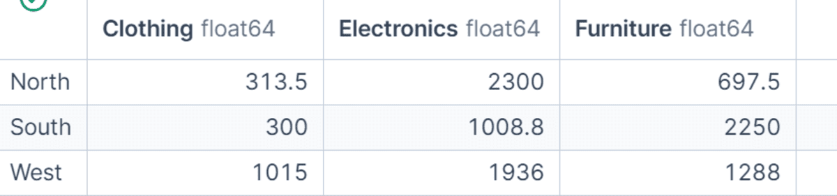
groupby() と unstack() を組み合わせることで、ピボット形式の要約テーブルを作成することができます。
この例では、データを地域とカテゴリでグループ化し、ネット販売高の合計を計算した上で、結果を再構成してカテゴリを列として表示します。これにより、地域やカテゴリ間での出力比較が容易になります。レポート作成や迅速な分析のためにコンパクトな表が必要な場合に非常に有効なテクニックです。
region_category_table = (
    df.groupby(["region", "category"])["net_sales"]
      .sum()
      .unstack(fill_value=0)
)

region_category_table
# 結論
Pandas の GroupBy は、Python におけるデータ分析で最も強力なツールの一つです。不必要な手動ロジックを書かずに、データの要約、グループ間の比較、新特徴量の作成、結果のフィルタリング、カスタム計算の適用を可能にします。
このチュートリアルに取り組む中で、GroupBy には非常に深い奥行きがあることを実感しました。データ処理に何年も携わっていても、一般的な問題を解決するための新しいより良い方法を学ぶことができました。pd.Grouper、カスタム集約関数、transform() といった機能は、多くのタスクをより高速でクリーンかつ保守しやすくするため、特に際立っています。
これが、ネイティブツールを理解することがなぜ重要なのかという理由でもあります。バイブコーディングや即席のカスタムソリューションに頼りたくなるものですが、それらは往々にしてより遅く、より複雑なコードを生み出してしまいます。pandas がすでに提供している機能を知っていれば、より効率的で再利用可能、かつ実世界のデータ分析に適したソリューションを書くことができます。
本チュートリアルでは、基本的な集計、名前付き集計、複数カラムによるグループ化、ソート、count() と size() の違い、transform()、filter()、apply()、日付によるグループ化、ピボット形式の要約など、最も有用な GroupBy 操作を解説しました。これらのパターンを理解すれば、GroupBy を用いて多くの実世界のデータ分析質問に迅速かつ自信を持って回答できるようになります。
Abid Ali Awan ** (@1abidaliawan) は機械学習モデルの構築を愛する認定データサイエンティストです。現在、機械学習およびデータサイエンス技術に関するコンテンツ作成や技術ブログの執筆に注力しています。Abid はテクノロジー管理の修士号と通信工学の学士号を取得しており、精神疾患で苦しむ学生向けにグラフニューラルネットワークを用いた AI 製品を構築するというビジョンを持っています。
原文を表示
**
# Introduction
Pandas is one of the most popular Python libraries for data analysis. It gives you simple tools for cleaning, reshaping, summarizing, and exploring structured data. One of the most useful features in pandas is GroupBy**. It helps you answer questions that require grouping rows by one or more categories.
For example, if you are working with sales data, you may want to calculate total revenue by region, average order value by product category, or the number of orders handled by each sales representative. Instead of manually filtering each category one by one, GroupBy lets you perform these calculations in a clean and efficient way.
In this tutorial, we will walk through practical examples of using Pandas GroupBy with a small sales dataset. I am using Deepnote as the coding environment, so some outputs are shown as notebook screenshots directly under the code blocks.
# Creating a Sample Dataset
**
Before using GroupBy, we first create a small retail sales dataset with columns such as order_id, region, category, sales_rep, units, unit_price, discount, and order_date. We then convert the dictionary into a pandas DataFrame and create two new columns: gross_sales and net_sales.
data = {
"order_id": [101, 102, 103, 104, 105, 106, 107, 108, 109, 110, 111, 112],
"region": ["North", "South", "North", "West", "South", "West", "North", "South", "West", "North", "South", "West"],
"category": ["Electronics", "Furniture", "Electronics", "Furniture", "Clothing", "Electronics",
"Clothing", "Furniture", "Clothing", "Furniture", "Electronics", "Clothing"],
"sales_rep": ["Ayesha", "Bilal", "Ayesha", "Chen", "Bilal", "Chen",
"Ayesha", "Bilal", "Chen", "Ayesha", "Bilal", "Chen"],
"units": [2, 1, 3, 2, 5, 4, 6, 2, 7, 1, 2, 8],
"unit_price": [500, 800, 450, 700, 60, 550, 55, 850, 65, 750, 520, 70],
"discount": [0.05, 0.10, 0.00, 0.08, 0.00, 0.12, 0.05, 0.10, 0.00, 0.07, 0.03, 0.00],
"order_date": pd.to_datetime([
"2026-01-05", "2026-01-06", "2026-01-08", "2026-01-10",
"2026-01-12", "2026-01-15", "2026-02-02", "2026-02-05",
"2026-02-08", "2026-02-12", "2026-02-15", "2026-02-20"
])
}
df = pd.DataFrame(data)
df["gross_sales"] = df["units"] * df["unit_price"]
df["net_sales"] = df["gross_sales"] * (1 - df["discount"])
dfThe gross_sales column is calculated by multiplying units by unit_price, while net_sales adjusts that value after applying the discount. This gives us a clean dataset that we can use for all GroupBy examples.
# Using the Basic GroupBy Syntax
The most basic GroupBy operation follows a simple pattern: select a grouping column, select the value column, and apply an aggregation function. In this example, we group the data by region and calculate the total net_sales for each region.
df.groupby("region")["net_sales"].sum()The result shows that North, South, and West each have their own total sales value. This is the simplest and most common use case for GroupBy when summarizing data.
region
North 3311.0
South 3558.8
West 4239.0
Name: net_sales, dtype: float64# Using GroupBy With as_index=False
By default, pandas uses the grouped column as the index in the output. While this is useful in some cases, it is often easier to work with a normal DataFrame where the grouped column remains a regular column. That is where as_index=False is useful.
df.groupby("region", as_index=False)["net_sales"].sum()In this example, we again calculate total net sales by region, but the result is returned as a clean DataFrame, which is easier to export, merge, or use in reports.
# Applying Multiple Aggregations on One Column
GroupBy is not limited to a single calculation. You can apply multiple aggregation functions to the same column using agg().
In this example, we calculate the sum, mean, minimum, maximum, and count of net_sales for each region.
This gives us a quick statistical summary of regional sales performance and helps us compare not only total revenue but also average order size and order volume.
df.groupby("region")["net_sales"].agg(["sum", "mean", "min", "max", "count"])# Using Named Aggregations
Named aggregations make GroupBy outputs easier to read and use. Instead of returning generic column names like sum or mean, we define our own names such as total_sales, average_order_value, total_units, and number_of_orders.
This is especially helpful when preparing analysis for dashboards, reports, or tutorials because the output column names clearly explain what each metric represents.
region_summary = (
df.groupby("region", as_index=False)
.agg(
total_sales=("net_sales", "sum"),
average_order_value=("net_sales", "mean"),
total_units=("units", "sum"),
number_of_orders=("order_id", "count")
)
)
region_summary# Grouping by Multiple Columns
You can also group data by more than one column. In this example, we group by both region and category to calculate total net sales for each product category within each region.
This gives us a more detailed view of the data compared to grouping by region alone. Multi-column grouping is useful when you want to analyze performance across different dimensions, such as region and product, department and employee, or month and customer segment.
df.groupby(["region", "category"], as_index=False)["net_sales"].sum()# Sorting GroupBy Results
After grouping and aggregating data, you often want to sort the results to find the highest or lowest values.
In this example, we calculate total sales by product category and then sort the results in descending order.
This makes it easy to identify which category generated the most revenue. Sorting grouped results is a simple but powerful step when turning raw summaries into useful insights.
category_sales = (
df.groupby("category", as_index=False)
.agg(total_sales=("net_sales", "sum"))
.sort_values("total_sales", ascending=False)
)
category_sales# Understanding Count vs Size
Pandas provides both count() and size(), but they are not exactly the same. The size() method counts the total number of rows in each group, including rows with missing values. The count() method counts only non-missing values in a selected column.
In this example, we intentionally add a missing value to the sales_rep column. The output shows that size() still counts four rows for each region, while count() returns three for North because one sales_rep value is missing.
import numpy as np
df_missing = df.copy()
df_missing.loc[2, "sales_rep"] = np.nan
print("Using size():")
display(df_missing.groupby("region").size())
print("Using count() on sales_rep:")
display(df_missing.groupby("region")["sales_rep"].count())Output:
Using size():
region
North 4
South 4
West 4
dtype: int64
Using count() on sales_rep:
region
North 3
South 4
West 4
Name: sales_rep, dtype: int64# Using transform() for Group-Level Features
The transform() method is useful when you want to calculate a group-level value and add it back to the original DataFrame.
In this example, we calculate total sales for each region and store it in a new column called region_total_sales.
We then calculate each order's share of its region's total sales. Unlike agg(), which reduces the data to one row per group, transform() returns values aligned with the original rows, making it very useful for feature engineering.
df["region_total_sales"] = df.groupby("region")["net_sales"].transform("sum")
df["order_share_of_region"] = df["net_sales"] / df["region_total_sales"]
df[["order_id", "region", "net_sales", "region_total_sales", "order_share_of_region"]]# Filtering Groups With filter()
The filter() method lets you keep or remove entire groups based on a condition. In this example, we keep only the regions where total net sales are greater than 3,000.
Instead of returning one summary row per group, filter() returns the original rows from the groups that meet the condition. This is useful when you want to remove low-performing groups or keep only groups that satisfy a business rule.
high_sales_regions = df.groupby("region").filter(lambda group: group["net_sales"].sum() > 3000)
high_sales_regions# Applying Custom Logic With apply()
The apply() method gives you more flexibility because it allows you to run custom logic on each group.
In this example, we use apply() with nlargest() to find the top order by net sales in each region. This is useful when built-in aggregation functions are not enough for your analysis.
However, apply() can be slower than built-in methods like sum(), mean(), agg(), and transform(), so it is best to use it only when you need custom group-wise operations.
top_order_by_region = (
df.groupby("region", group_keys=False)
.apply(lambda group: group.nlargest(1, "net_sales"))
)
top_order_by_region# Grouping by Dates
GroupBy is also very useful for time-based analysis.
In this example, we extract the month from the order_date column and group the data by month.
We then calculate total sales and total orders for each month. This approach is helpful when analyzing trends over time, such as monthly sales, weekly user activity, or yearly revenue growth.
df["month"] = df["order_date"].dt.to_period("M").astype(str)
monthly_sales = (
df.groupby("month", as_index=False)
.agg(total_sales=("net_sales", "sum"), total_orders=("order_id", "count"))
)
monthly_sales# Grouping by Dates With pd.Grouper
pd.Grouper provides a cleaner way to group time series data without manually creating a separate month column.
In this example, we group the DataFrame by order_date using a monthly frequency and calculate total sales and total orders.
This is especially useful when working with real-world datasets that contain timestamps and you want to summarize data by day, week, month, quarter, or year.
monthly_sales_grouper = (
df.groupby(pd.Grouper(key="order_date", freq="M"))
.agg(total_sales=("net_sales", "sum"), total_orders=("order_id", "count"))
.reset_index()
)
monthly_sales_grouper# Creating a Pivot-Style Summary With GroupBy
You can combine groupby() with unstack() to create a pivot-style summary table.
In this example, we group the data by region and category, calculate total net sales, and then reshape the result so that categories become columns. This makes the output easier to compare across regions and categories. It is a great technique when you want a compact table for reporting or quick analysis.
region_category_table = (
df.groupby(["region", "category"])["net_sales"]
.sum()
.unstack(fill_value=0)
)
region_category_table# Conclusion
Pandas GroupBy is one of the most powerful tools for data analysis in Python. It helps you summarize data, compare groups, create new features, filter results, and apply custom calculations without writing unnecessary manual logic.
While working on this tutorial, I realized how much depth there is in GroupBy. Even after working with data for years, I learned new and better ways to solve common problems. Features like pd.Grouper, custom aggregation functions, and transform() stood out because they make many tasks faster, cleaner, and easier to maintain.
This is also why understanding the native tools matters. It is tempting to rely on vibe coding or quick custom solutions, but those can often produce slower, more complicated code. When you know what pandas already provides, you can write solutions that are more efficient, reusable, and practical for real-world data analysis.
In this tutorial, we covered the most useful GroupBy operations, including basic aggregation, named aggregation, multi-column grouping, sorting, count() vs size(), transform(), filter(), apply(), date grouping, and pivot-style summaries. Once you understand these patterns, you can use GroupBy to answer many real-world data analysis questions quickly and confidently.
Abid Ali Awan** (@1abidaliawan) is a certified data scientist professional who loves building machine learning models. Currently, he is focusing on content creation and writing technical blogs on machine learning and data science technologies. Abid holds a Master's degree in technology management and a bachelor's degree in telecommunication engineering. His vision is to build an AI product using a graph neural network for students struggling with mental illness.
関連記事
Pandas でループを書かない:試すべき 7 つの高速代替案
KDnuggets は、Pandas データ処理でループを使用する代わりに、ベクトル化や組み込み関数など 7 つの高速な代替手法を紹介している。
データクリーニングと前処理のための Pandas の 3 つの技
KDnuggets が紹介する記事で、Pandas ライブラリを用いたデータクリーニングと前処理を効率化する 3 つの実用的なテクニックが解説されています。
datasette-acl 0.6a0 のリリース
Alex Garcia 氏らが中心となり、データセットのテーブル単位での権限管理から、一般リソース共有システムへと拡張された「datasette-acl」バージョン 0.6a0 が公開されました。これにより、複数ユーザー環境でリソースへのアクセス制御が細かく行えるようになります。
今日のまとめ
AI日報で今日の重要ニュースをまとめ読み