機械学習ワークフローのための可視化デバッグツール
本記事は、機械学習モデルのトレーニング中に発生する過学習や学習不足などの問題を特定するために、勾配・損失・埋め込みベクトルを可視化するツールと手法について解説している。
キーポイント
損失曲線と勾配フローの重要性
トレーニングと検証の損失曲線の乖離(過学習)や早期の頭打ち(学習不足)を視覚的に確認し、勾配消失問題の兆候を検出する基礎的な手法を解説している。
主要可視化ツールの紹介
TensorBoard を中心に、モデル内部の状態を可視化するための代替ツールや、その基本的な機能について言及されている。
フックとブレークポイントによる直接計測
標準的なログ出力に加え、フック(hooks)やデバッグブレイクポイントを使用してモデル計算を直接キャプチャ・解析する高度な手法について触れている。
Loss Curvesによるモデル診断
訓練損失と検証損失の推移を監視することで、過学習(検証損失の上昇)や学習不足(両者の早期プラトー)、勾配消失問題(損失の緩やかな低下)を検出できます。
層ごとの勾配マグニチュード可視化
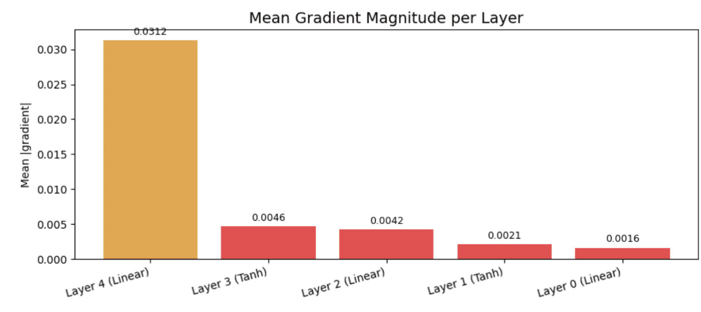
各層の平均勾配絶対値をプロットすることで、勾配が早期の層で小さくなりすぎている(消失している)具体的な箇所を特定し、アーキテクチャや学習率の問題を調査できます。
勾配消失問題の可視化
各層の勾配値をプロットすることで、初期層での勾配が急激に減少し学習が遅くなる「勾配消失問題」を検出できます。
PyTorch を用いた実装方法
`register_backward_hook` 関数を使用すれば、トレーニングループを変更せずに任意の層から勾配テンソルを取得し可視化可能です。
重要な引用
What most analysts skip at this stage is actual visibility into what is happening inside the model during training.
When validation loss starts rising while training loss keeps falling, the model is overfitting.
The vanishing gradient problem may manifest in practice if the loss curves decrease smoothly but too slowly.
The red bar that appears on each of the first three layers indicates that gradients are already in the risk zone before they ever reach the start of the network.
What we're looking for in a healthy network is histograms across layers with roughly similar spreads.
If the classes are tight and well-separated, that means the model has learned useful separation.
影響分析・編集コメントを表示
影響分析
この記事は、機械学習エンジニアがモデルの挙動をブラックボックスとして扱うのではなく、可視化ツールを活用して内部状態を解明する重要性を再認識させる内容です。特に、過学習や勾配消失といった一般的な問題に対する具体的な診断手法を提供することで、開発効率の向上とモデル改善の精度向上に寄与します。
編集コメント
モデル開発の現場では、数値結果だけでなく「なぜそうなるのか」を可視化で確認する習慣が欠如しているケースが多々あります。本記事は、そのギャップを埋めるための具体的なツールとアプローチを提供しており、実務におけるデバッグスキル向上に役立つ良質なコンテンツです。
**
# イントロダクション
機械学習モデルのトレーニングを行い、損失(loss)が減少する様子を観察することは進歩を実感できる瞬間ですが、検証精度が頭打ちになったり、損失が急上昇し始めたりしたときに、その原因が不明だと途方に暮れることになります。そのような局面では、多くの人がより多くのログを追加するか、ハイパーパラメータの調整を始め、何かが変わることを願うものです。しかし、この段階で多くの分析者が見落としているのは、トレーニング中にモデル内部で何が起きているのかを直接可視化する視点です。ビジュアルデバッグツールは、この段階で有用な洞察を提供できます。
本記事では、3 つのトピックを取り上げます:トレーニング中に何を可視化すべきか(勾配、損失、埋め込み)、それらの可視化を実現するツール(TensorBoard とその主要な代替手段)、およびフックやブレークポイントを使用してモデルの計算を直接キャプチャする方法です。
**
# 勾配、損失、埋め込みの可視化
// 損失曲線
モデルのトレーニングを行う際、損失曲線は通常最初に確認すべき項目です。トレーニング損失と検証損失の両方が低下し、互いに近い値で推移している場合は、トレーニングが順調に進んでいることを示します。一方、検証損失の上昇が始まりながらトレーニング損失がさらに低下する場合は、モデルが過学習を起こしています。また、両方の曲線が早期に頭打ちになる場合、モデルが学習できていないことを意味し、これは通常データまたは学習率に問題があることを示唆します。
加えて、勾配の流れも重要です。損失曲線が滑らかに減少しているにもかかわらず、非常に遅い場合は、実務において勾配消失現象が発生している可能性があります。これは、勾配が初期層に到達するまでに小さくなりすぎていることを示しています。
以下に示すプロットは、典型的な過学習パターンをシミュレーションしたものです。最初の 10 エポックでは両方の損失が同時に減少しますが、その後、検証損失の上昇が始まりながらトレーニング損失はさらに低下し続けます。
赤い点線は分岐が始まる地点を示しています:実際のランでは、これが正則化や早期打ち切りを検討すべきポイントとなります。
import torch
import torch.nn as nn
import matplotlib.pyplot as plt

model = nn.Sequential(nn.Linear(16, 16), nn.Tanh(),
                      nn.Linear(16, 16), nn.Tanh(),
                      nn.Linear(16, 1))

grad_magnitudes = {}

def grad_hook(name):
    def hook(module, grad_input, grad_output):
        grad_magnitudes[name] = grad_output[0].abs().mean().item()
    return hook

for i, layer in enumerate(model):
    layer.register_backward_hook(grad_hook(f"Layer {i}"))
output = model(torch.randn(32, 16))
output.mean().backward()
plt.bar(grad_magnitudes.keys(), grad_magnitudes.values())
plt.title("Mean Gradient Magnitude per Layer")
plt.ylabel("Mean |gradient|")
plt.xticks(rotation=15)
plt.tight_layout()
plt.show()
It outputs:
// Raw Gradient Magnitudes
Layer 4 (Linear): 0.031250
Layer 3 (Tanh): 0.004646
Layer 2 (Linear): 0.004241
Layer 1 (Tanh): 0.002126
Layer 0 (Linear): 0.001631
The chart reads right to left: Layer 4 represents the output layer, and Layer 0 is the first. The output layer gets a gradient of 0.031, but by the time it reaches Layer 0, that number has dropped to 0.0016 — roughly 20 times smaller.
The red bar that appears on each of the first three layers indicates that gradients are already in the risk zone before they ever reach the start of the network. In a real training run on a deeper model, these initial layers would adjust their weights so slowly that they would hardly learn anything.
This is a practical example of the vanishing gradient problem: the early layers are silently undertraining, which can't be seen without this kind of plot.
トレーニング中に層ごとに勾配の大きさをプロットすることで、勾配がネットワークの初期部分に十分な値を持って到達しているかどうかを直接確認できます。深層モデルでは、勾配が層を遡って移動する際に消失することがあります。トレーニング中に記録された各層の勾配値ヒストグラムはこのパターンを明らかにし、問題を早期に特定するのに役立ちます。
PyTorch の register_backward_hook 関数を使用すると、トレーニングループを変更することなく、任意の層から勾配テンソルを取得できます。モジュールにフックを接続することで、各バックワードパス時に活性化し、勾配テンソルを指定されたコールバックに送信します。
以下のヒストグラムは、1 回のバックワードパス後に各層の勾配値の完全な分布を示しています。各サブプロットは単一の層を表しており、初期層から最終層へと順に並んでいます。
このコードは こちら で確認できます。
**
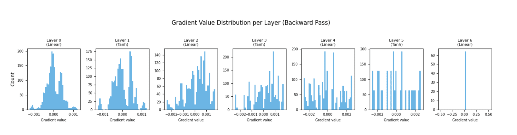
健全なネットワークで目指すべきは、層全体にわたってほぼ同程度の広がりを持つヒストグラムです。
もし初期層がゼロを中心に非常に狭くスパイク状の分布を示す場合、それは勾配消失(vanishing gradients)を示す危険信号となる可能性があります。
勾配はまだ存在しますが、非常に小さく、ほとんど学習情報を運んでいません。この可視化により、完全なトレーニング実行後ではなく、最初の数バッチの後にこのパターンを検出できます。
// Embeddings
モデルが入力を学習された表現にマッピングする場合、その表現を可視化することで、モデルが期待通りにデータを分離できているかどうかを確認できます。最も一般的なアプローチは、訓練済み(または部分的に訓練済み)モデルからの埋め込みを取得し、t-SNE または UMAP を使用して次元削減を行い、クラスラベルを色としてプロットすることです。
クラスが密で明確に分離されている場合、モデルが有用な分離を学習したことを意味します。クラスが重なっている場合は、モデルがまだ概念を分離できていないことを示します。このステップは、最終的な分類層を追加する前に、テキストや画像でトレーニングされたモデルのデバッグに役立ちます。
# TensorBoard and Its Alternatives
**
// TensorBoard
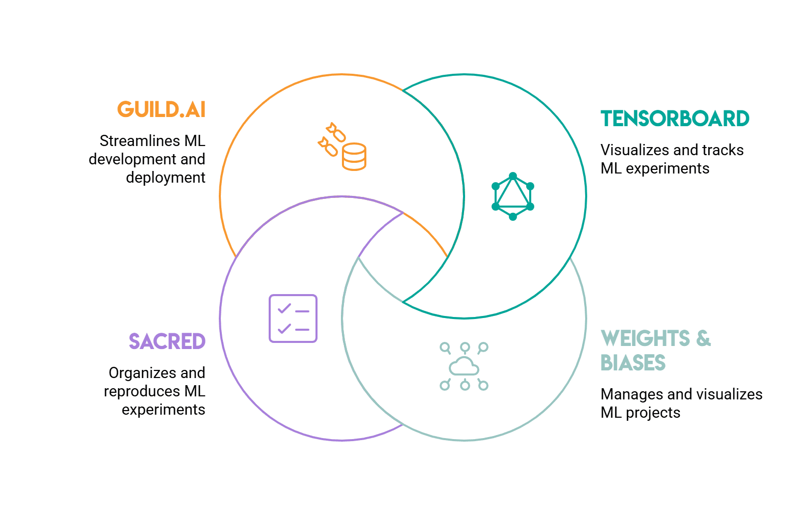
TensorBoard は標準的な出発点です。元々は TensorFlow のために構築されましたが、torch.utils.tensorboard を通じて PyTorch でも動作します。データは SummaryWriter オブジェクトを通じてログに記録され、ブラウザのタブで結果を確認できます。スカラー値(損失、精度)、ヒストグラム(重みと勾配の分布)、画像、および高次元表現を可視化するための埋め込みプロジェクターを処理します。
主な制限はローカリティにあります。チームと結果を共有するには、ログファイル用の共有ストレージを設定するか、TensorBoard.dev を使用する必要がありますが、そこにはサポートされる内容に制限があります。
// Weights & Biases
Weights & Biases (W&B) は、多くの機械学習チームがコラボレーションやより詳細な追跡のために使用するツールです。
セットアップは 2 行で完了します。ランの開始時に wandb.init() を実行し、トレーニングループ内で wandb.log() を呼び出します。すべてのデータが自動的にクラウドダッシュボードに同期され、プロジェクトごとにランがグループ化されるため、実験の比較が容易になります。
以下のコードスニペットを確認してください:
import wandb

wandb.init(project="my-model", config={"lr": 0.001, "epochs": 20, "batch_size": 32})

for epoch in range(wandb.config.epochs):
    train_loss = 1 / (1 + 0.3 * epoch)   # simulated
    val_loss   = train_loss + max(0, 0.04 * (epoch - 10))  # simulated
    wandb.log({"epoch": epoch, "train_loss": train_loss, "val_loss": val_loss})

wandb.finish()
実行が完了すると、W&B ダッシュボード上で、それらを生成した設定と共に記録されたメトリクスを確認できます。異なるパラメータを持つ 2 つの実行を比較する際も、インターフェースでそれらを選択するだけで済み、手動でのログ解析は不要です。
W&B は、ハイパーパラメータスイープにも組み込みの可視化機能をサポートしており、どのハイパーパラメータが結果に最も大きな影響を与えたかを示します。
GPU 利用率やメモリ使用量などのシステムメトリクスも自動的に記録されます。並列で多数の実験を実行するチームにとって、共有ワークスペースにより、何を試したかを追跡するための手作業の負担を大幅に軽減できます。
// Sacred
Sacred は異なるアプローチを採用しています。これは可視化よりも再現性に焦点を当てています。トレーニングスクリプトに Sacred の実験デコレータを注釈付けすることで、設定全体、実行中のあらゆる変更、および記録されたすべてのメトリクスがデータベース(通常は MongoDB)に記録されます。これにより、各実行とその正確な設定が恒久的な記録となります。
可視化については、Sacred は Omniboard や Sacredboard などのフロントエンドと連携します。TensorBoard や W&B に比べると複雑さが増しますが、その強みは監査可能性にあります:過去のいかなる実行も、当初の設定通りに正確に再現可能です。
// Guild.ai
Guild.ai はコマンドラインから動作し、トレーニングコードを変更する必要はありません。guild run train.py を使用して Guild でトレーニングスクリプトを実行すると、スクリプトが生成するすべてのログと出力ファイルが記録され、それらが特定のランに関連付けられます。メトリクスやランの比較は、Guild のコマンドラインインターフェース (CLI) またはローカル UI を通じて利用可能です。
このフレームワークは、既存のスクリプトや修正したくないサードパーティ製コードを扱う場合に適しています。W&B に比べると機能は少ないものの、セットアップコストも低いです。
# 機械学習計算におけるブレークポイントとフックの使用
// フォワードおよびバックワードフック
PyTorch のフックシステムを使用すると、モデルのフォワードパスまたはバックワードパス内の任意の時点で計算をインターセプトできます。register_forward_hook 関数は、任意のレイヤーにコールバックをアタッチし、そのレイヤーがバッチを処理するたびに発火します。このコールバックは、レイヤーの入力および出力テンソルをキャプチャするため、これらをログ記録したり、NaN 値をチェックしたり、プロットしたりできます。
register_backward_hook 関数は、バックワードパスに対して同様の役割を果たし、各層を流れる勾配テンソルへのアクセスを提供します。これら 2 つのフックを組み合わせることで、モデル定義やトレーニングループを変更することなく、トレーニング中に検査したいことのほとんどをカバーできます。
実用的な応用例として、NaN(Not a Number)値の検出があります。各層の出力で tensor.isnan().any() を評価するフォワードフックを使用することで、数値的不安定性を即座に検出し、それが拡散してトレーニングの残りを損なうのを防ぐことができます。
以下は、各層にフックを付けた 3 層モデルを使用した最小限の実行例です:
import torch
import torch.nn as nn
model = nn.Sequential(nn.Linear(8, 16), nn.ReLU(), nn.Linear(16, 4))
def nan_hook(layer, input, output):
if output.isnan().any():
print(f"[NaN detected] Layer: {layer.__class__.__name__}")
else:
print(f"[Clean] Layer: {layer.__class__.__name__}, output shape: {tuple(output.shape)}")
for layer in model:
layer.register_forward_hook(nan_hook)
print("--- Normal input ---")
model(torch.randn(2, 8))
print("\n--- Corrupted input ---")
bad_input = torch.randn(2, 8)
bad_input[0, 3] = float('nan')
model(bad_input)
実行時の期待される出力:
--- Normal input ---
[Clean] Layer: Linear, output shape: (2, 16)
[Clean] Layer: ReLU, output shape: (2, 16)
[Clean] Layer: Linear, output shape: (2, 4)
--- Corrupted input ---
[NaN detected] Layer: Linear
[NaN detected] Layer: ReLU
[NaN detected] Layer: Linear
この例では、フックは各層が実行された後の出力テンソルをチェックし、それが正常か破損しているかを報告します。
これを 2 回実行する — 1 回は通常の入力で行い、もう 1 回は単一の NaN を注入して行うことで、不安定性がネットワーク内でどのように層ごとに伝播するかを示すことができます。
// デバッガーのブレークポイント
標準的な Python デバッガーは、トレーニングループ内でも十分に機能します。
任意の箇所に import pdb; pdb.set_trace() を挿入して実行を一時停止し、インタラクティブなプロンプトを表示させることで、テンソルの形状を確認したり、データ前処理が予期しない値を生み出していないかを検証したり、手動で順伝播(フォワードパス)をステップ実行したりすることが可能です。
VSCode や PyCharm といった、ほとんどの機械学習開発環境では、グラフィカルにブレークポイントを設定し、専用パネルでテンソルを検査できるため、ターミナルベースの pdb インターフェースよりも迅速な代替手段を提供しています。
ただし、ブレークポイントは、完全なトレーニング実行を開始する前にデータ、モデル、損失関数が適切に動作していることを確認するために、最初の 1〜2 バッチの間特に有用です。
# 結論
**
内部で何が起きているかを可視化せずにモデルを訓練することは、実際の原因ではなく症状を解釈することにほかなりません。
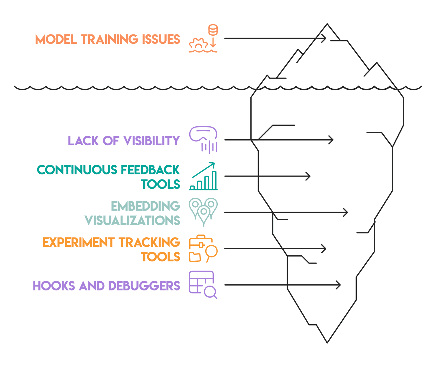
モデルを訓練する際、損失曲線が早期に頭打ちになる、勾配が消滅する、あるいは埋め込み表現が分離しないといった現象が起きたとしても、適切な計測(インストルメンテーション)が行われていなければ、これらの要因は明確に自らを主張することはありません。
この記事で紹介されたツールは、それぞれ異なるレベルで機能します。損失曲線や勾配ヒストグラムはトレーニング中に継続的なフィードバックを提供し、過学習や勾配消失といった問題が蓄積してフレームワークを破綻させる前に検出します。
埋め込み可視化は、モデルがデータから適切な分離を学習できているかを示します。TensorBoard、W&B、Sacred、Guild.ai はそれぞれログ記録と追跡の側面を異なる方法で扱いますが、すべて同じ目的を果たしています。つまり、実験履歴を散らかった状態ではなく、検索可能かつ比較可能なものにするのです。最後に、フックやデバッガーはさらに一歩進んで、ネットワーク内の任意のレイヤーを流れる実際のテンソルを一時停止して検査することを可能にします。
ただし、これらのツール単独で壊れたモデルを修復することはできません。それらが果たすのは、問題が発生した原因を理解するまでの距離を短縮することです。これは通常、作業の大部分を占める部分です。
Nate Rosidi** はデータサイエンティストであり、製品戦略にも携わっています。また、分析を教える非常勤教授でもあり、トップ企業からの実際の面接質問を用いてデータサイエンティストの面接準備をサポートするプラットフォーム「StrataScratch」の創設者です。Nate はキャリア市場における最新動向について執筆し、面接に関するアドバイスを提供し、データサイエンスプロジェクトを紹介し、SQL 関連のあらゆるトピックをカバーしています。
原文を表示

**
# Introduction
Training a machine learning model and observing the loss decrease is a feeling of progress, until the validation accuracy reaches a plateau or the loss begins to spike, and you're not sure what caused it. At that point, most people add more logging or start tuning hyperparameters, hoping something changes. What most analysts skip at this stage is actual visibility into what is happening inside the model during training. Visual debugging tools can provide useful insights at this stage.
In this article, we cover three topics: what to visualize during training (gradients, losses, and embeddings), the tools that provide those visualizations (TensorBoard** and its main alternatives), and the methods to capture model computations directly using hooks and breakpoints.
**
# Visualizing Gradients, Losses, and Embeddings
// Loss Curves
When training a model, the loss curve is usually the first thing to check. When both the training loss and validation loss decline and remain close, it indicates that the training is progressing well. When validation loss starts rising while training loss keeps falling, the model is overfitting. When both curves plateau early, the model isn't learning, which typically indicates a problem with the data or learning rate.
In addition, gradient flow is also important. The vanishing gradient problem may manifest in practice if the loss curves decrease smoothly but too slowly, indicating that gradients are too small by the time they reach early layers.
The plot shown below simulates a typical overfitting pattern. Both losses decrease together for the first ten epochs, and then the validation loss starts increasing while the training loss keeps falling.
The red dotted line marks where the divergence begins: in a real run, that's the point to start investigating regularization or early stopping.
import torch
import torch.nn as nn
import matplotlib.pyplot as plt

model = nn.Sequential(nn.Linear(16, 16), nn.Tanh(),
                      nn.Linear(16, 16), nn.Tanh(),
                      nn.Linear(16, 1))

grad_magnitudes = {}

def grad_hook(name):
    def hook(module, grad_input, grad_output):
        grad_magnitudes[name] = grad_output[0].abs().mean().item()
    return hook

for i, layer in enumerate(model):
    layer.register_backward_hook(grad_hook(f"Layer {i}"))

output = model(torch.randn(32, 16))
output.mean().backward()

plt.bar(grad_magnitudes.keys(), grad_magnitudes.values())
plt.title("Mean Gradient Magnitude per Layer")
plt.ylabel("Mean |gradient|")
plt.xticks(rotation=15)
plt.tight_layout()
plt.show()
It outputs:
// Raw Gradient Magnitudes
Layer 4 (Linear): 0.031250
Layer 3 (Tanh): 0.004646
Layer 2 (Linear): 0.004241
Layer 1 (Tanh): 0.002126
Layer 0 (Linear): 0.001631
The chart reads right to left: Layer 4 represents the output layer, and Layer 0 is the first. The output layer gets a gradient of 0.031, but by the time it reaches Layer 0, that number has dropped to 0.0016 — roughly 20 times smaller.
The red bar that appears on each of the first three layers indicates that gradients are already in the risk zone before they ever reach the start of the network. In a real training run on a deeper model, these initial layers would adjust their weights so slowly that they would hardly learn anything.
This is a practical example of the vanishing gradient problem: the early layers are silently undertraining, which can't be seen without this kind of plot.
// Gradient Visualization
Plotting gradient magnitudes layer by layer during training gives a direct view of whether gradients are reaching the early parts of the network with considerable values. In deep models, gradients may vanish as they move backward through layers. The gradient value histograms for each layer, recorded during training, can reveal this pattern and help us identify the issue early on.
PyTorch**'s register_backward_hook function allows us to obtain gradient tensors from any layer without modifying the training loop. We connect a hook to a module, which activates during each backward pass, sending the gradient tensors to a specified callback.
The histogram below shows the complete distribution of gradient values for each layer after one backward pass. Each subplot represents a single layer, ordered from the initial layer to the final one.
The code for this can be found here.
**
What we're looking for in a healthy network is histograms across layers with roughly similar spreads.
If the early layers show a very narrow, spike-like distribution centered tightly on zero, that could be a red flag indicating vanishing gradients.
The gradients still exist, but they're so small they carry almost no learning information. This visualization can help us catch this pattern after the first few batches, rather than after a full training run.
// Embeddings
When a model maps inputs to a learned representation, visualizing that representation tells us whether the model is separating the data as we'd expect. The most common approach is to take the embeddings from a trained (or partially trained) model, reduce their dimensionality using t-SNE or UMAP**, and plot them with class labels as colors.
If the classes are tight and well-separated, that means the model has learned useful separation. Overlapping classes mean the model hasn't separated the concepts yet. This step is useful for debugging models trained on text or images before adding the final classification layer.
# TensorBoard and Its Alternatives
**
// TensorBoard
TensorBoard is your standard starting point. Originally built for TensorFlow**, it works with PyTorch through torch.utils.tensorboard. Data can be logged through a SummaryWriter object, and you can view the results in a browser tab. It handles scalars (loss, accuracy), histograms (weight and gradient distributions), images, and an embedding projector for visualizing high-dimensional representations.
The main limitation is its locality. Sharing your results with a team means setting up shared storage for log files or using TensorBoard.dev, which has limits on what it supports.
// Weights & Biases
Weights & Biases (W&B) is what most machine learning teams use for collaboration or more detailed tracking.
Setup is done with two lines: wandb.init() at the start of a run and wandb.log() inside the training loop. Everything syncs to a cloud dashboard automatically, and runs are grouped by project, making experiment comparison straightforward.
Check the code snippet below:
import wandb

wandb.init(project="my-model", config={"lr": 0.001, "epochs": 20, "batch_size": 32})

for epoch in range(wandb.config.epochs):
    train_loss = 1 / (1 + 0.3 * epoch)   # simulated
    val_loss   = train_loss + max(0, 0.04 * (epoch - 10))  # simulated
    wandb.log({"epoch": epoch, "train_loss": train_loss, "val_loss": val_loss})

wandb.finish()
Once the run finishes, the logged metrics can be viewed in the W&B dashboard, alongside the configuration that produced them. Comparing two runs with different parameters can easily be done by selecting them in the interface, with no manual log parsing needed.
W&B also supports hyperparameter sweeps with built-in visualization, showing which hyperparameters affected the outcome the most.
System metrics like GPU utilization and memory usage are also logged automatically. For teams running many experiments in parallel, the shared workspace removes a lot of the manual overhead of keeping track of what was tried.
// Sacred
Sacred takes a different approach. It focuses on reproducibility rather than visualization. We annotate a training script with Sacred's experiment decorator, which records the entire configuration, any changes made during runtime, and all recorded metrics in a database (usually MongoDB). This way, each run and its precise settings turn into a permanent record.
For the visualization part, Sacred pairs with front-ends like Omniboard or Sacredboard. This adds complexity compared to TensorBoard or W&B, but the strength is auditability: any run from the past can be reproduced exactly as it was configured.
// Guild.ai
Guild.ai works from the command line and doesn't require you to change the training code. We run a training script through Guild using guild run train.py, which records all the logs produced by the script along with any output files, linking them to that particular run. Metrics and run comparisons are available through Guild's command-line interface (CLI) or its local UI.
This framework is a good choice when working with existing scripts or third-party code that we prefer not to modify. It provides fewer features than W&B, but the setup cost is also lower.
# Using Breakpoints and Hooks for Machine Learning Computations
// Forward and Backward Hooks
PyTorch's hook system lets us intercept computations at any point in a model's forward or backward pass. The register_forward_hook function attaches a callback to any layer, and it fires every time that layer processes a batch. The callback captures the layer's input and output tensors, which we can then log, check for NaN values, or plot.
The register_backward_hook function does the same for the backward pass, giving us access to the gradient tensors flowing through each layer. Together, these two hooks cover most of what we'd want to inspect during training without modifying the model definition or the training loop.
A practical application is the detection of NaN values. A forward hook that evaluates tensor.isnan().any() at every layer's output detects numerical instability right away, preventing it from spreading and damaging the rest of the training.
Here's a minimal working example, using a three-layer model with a hook attached to each layer:
import torch
import torch.nn as nn

model = nn.Sequential(nn.Linear(8, 16), nn.ReLU(), nn.Linear(16, 4))

def nan_hook(layer, input, output):
    if output.isnan().any():
        print(f"[NaN detected] Layer: {layer.__class__.__name__}")
    else:
        print(f"[Clean] Layer: {layer.__class__.__name__}, output shape: {tuple(output.shape)}")

for layer in model:
    layer.register_forward_hook(nan_hook)

print("--- Normal input ---")
model(torch.randn(2, 8))

print("\n--- Corrupted input ---")
bad_input = torch.randn(2, 8)
bad_input[0, 3] = float('nan')
model(bad_input)
Expected output when run:
--- Normal input ---

[Clean] Layer: Linear, output shape: (2, 16)
[Clean] Layer: ReLU, output shape: (2, 16)
[Clean] Layer: Linear, output shape: (2, 4)

--- Corrupted input ---

[NaN detected] Layer: Linear
[NaN detected] Layer: ReLU
[NaN detected] Layer: Linear
In this example, the hook checks the output tensor after each layer fires and reports whether it's clean or corrupted.
Running it twice — once with normal input and once with a single NaN injected — demonstrates how instability propagates through the network, layer by layer.
// Debugger Breakpoints
Standard Python debuggers work fine inside training loops.
Dropping import pdb; pdb.set_trace() at any point pauses execution and brings up an interactive prompt that allows us to examine tensor shapes, verify that data preprocessing hasn't produced unexpected values, and manually step through the forward pass.
Most machine learning development environments — VSCode and PyCharm both — let us set breakpoints graphically and inspect tensors in a dedicated pane, offering a quicker alternative to the terminal-based pdb interface.
However, breakpoints are particularly valuable during the initial one or two batches, as we confirm that the data, model, and loss function are working properly before starting a complete training run.
# Conclusion
**
Training a model without visualizing what's happening inside means interpreting symptoms rather than the actual causes.
When training a model, whether the loss curve plateaus early, gradients vanish, or embeddings don't separate, without the right instrumentation, none of these factors announce themselves clearly.
The tools covered in this article operate at different levels. Loss curves and gradient histograms give continuous feedback during training, catching problems like overfitting or vanishing gradients before they compound and break your framework.
Embedding visualizations reveal whether the model is learning a good separation from the data. TensorBoard, W&B, Sacred, and Guild.ai each handle the logging and tracking side differently, but they all serve the same purpose: making experiment history searchable and comparable rather than scattered. Finally, hooks and debuggers go one step further and let you pause and inspect the actual tensors flowing through the network at any layer.
Nonetheless, these tools can't fix a broken model on their own. What they do is shorten the distance between something going wrong and understanding why — which is usually most of the work.
Nate Rosidi** is a data scientist and in product strategy. He's also an adjunct professor teaching analytics, and is the founder of StrataScratch, a platform helping data scientists prepare for their interviews with real interview questions from top companies. Nate writes on the latest trends in the career market, gives interview advice, shares data science projects, and covers everything SQL.
関連記事
今日のまとめ
AI日報で今日の重要ニュースをまとめ読み