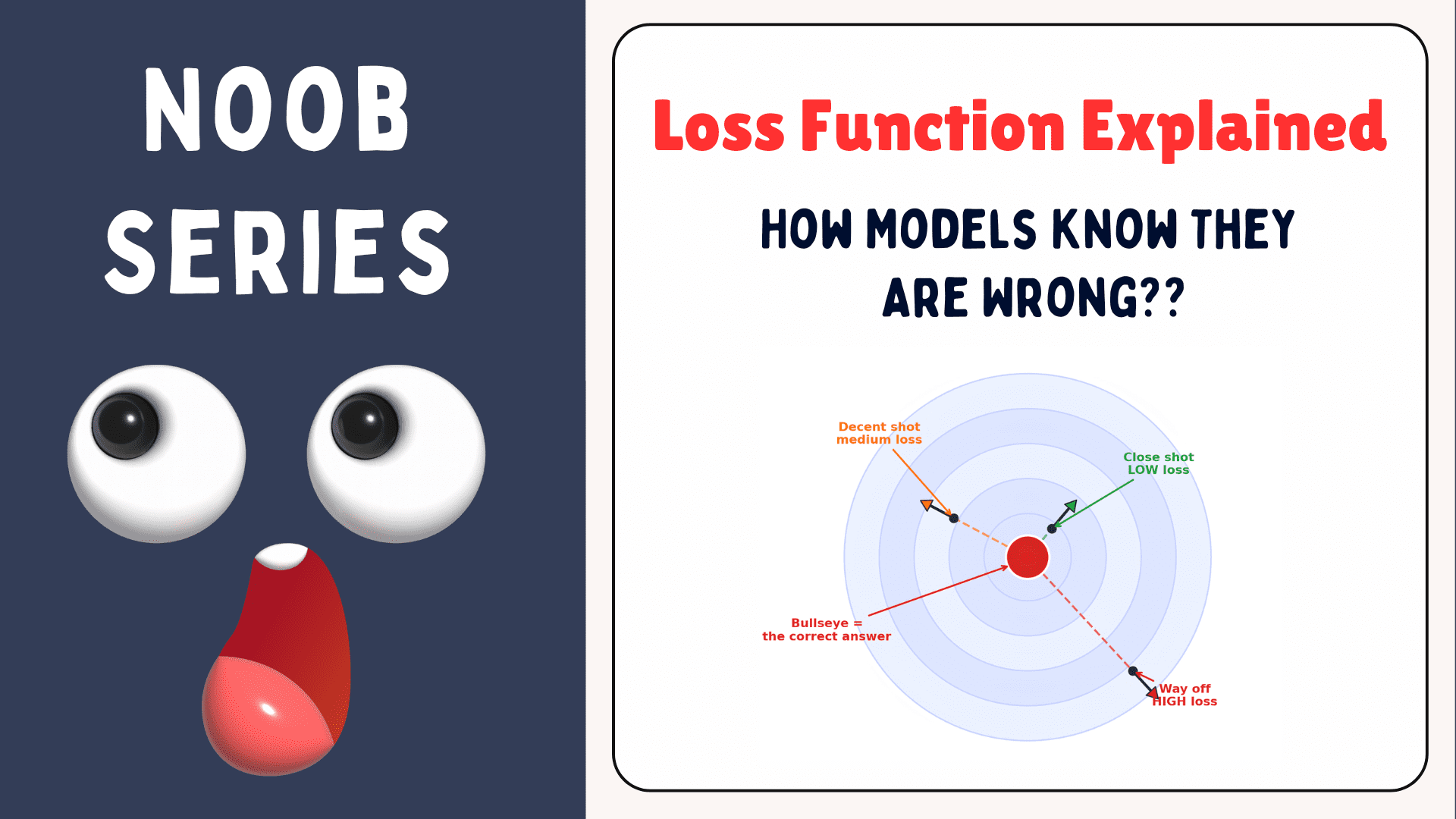
初心者のための損失関数解説(モデルが誤りをどう知るか)
KDnuggets は、機械学習モデルが誤りを認識し学習する基盤となる「損失関数」の概念を、初心者向けに分かりやすく解説している。
キーポイント
損失関数の定義と役割
予測値と正解ラベルとの差(誤差)を定量化し、モデルが「どれくらい間違っているか」を数値として示す指標である。
学習プロセスにおける機能
バックプロパゲーションの基礎となり、損失関数の値を最小化するように重みパラメータを更新する方向性を決定する。
代表的な損失関数の種類
回帰問題には平均二乗誤差(MSE)、分類問題には交差エントロピー(Cross-Entropy)など、タスクに応じて適切な関数を選択する必要がある。
初心者への教育的意義
複雑な数学的導出を避け、直感的な例を用いることで、AI 開発の初学者がモデル学習の核心を理解する手助けとなる。
影響分析・編集コメントを表示
影響分析
この記事は、AI 業界において基礎概念を再確認する価値のある教育的コンテンツであり、特に新規参入者や非技術系ステークホルダーにとって機械学習の動作原理を理解するための重要な入り口となる。損失関数の理解が不十分であるとモデル設計の誤りが生じるため、その重要性を広く周知させる効果がある。
編集コメント
高度な数式解説を避け、直感的な理解を優先した構成は、AI 業界の裾野を広げる上で非常に有益です。基礎固めが必要な層へのリーチに特化した良質な記事と言えます。
 image**
# イントロダクション
初心者が機械学習の学習を始めたとき、最初はすべてが簡単に見えるものだということは知っています。データセットを読み込み、モデルを訓練するよう指示されたチュートリアルに従うと、このような表示が出ます:loss = "mse" または criterion = nn.CrossEntropyLoss()。
そしてあっという間に、そのチュートリアルは数式や勾配、最適化、ギリシャ文字について話し始めます。損失関数が何をするのかを本当に理解せずに頷いた経験があるなら、あなた一人ではありません。損失関数の説明は往々にして逆から行われます。** ほとんどのチュートリアルは、まずアイデアから始めるべきところを、いきなり数式から始めてしまいます。この記事は私の「初心者向けシリーズ」の一部で、よりわかりやすく解説していきます。では、始めましょう。
# 損失関数とは何か?
損失関数は、機械学習モデルが自分がどれだけ間違っているかを把握する方法です。 これがまさに概念のすべてです。モデルが予測を行います。損失関数がその予測と正解を比較します。そして、「あなたの間違いはこれほどひどかった」という数をモデルに返します。
損失が高いということは、モデルが非常に間違っていたことを意味します。
損失が低いということは、モデルが近いことを意味します。
訓練中、モデルは損失を小さくするように自らを調整し続けます。
これが学習が行われる仕組みです。ダーツゲームをしたことがあるなら、非常に似ています。あなたはダーツを投げます。改善するためにはフィードバックが必要です。あなたのダーツがわずかに外れたのか、遠くにあるのか、高すぎたのか、あるいは左にやりすぎたのかを知る必要があります。そのフィードバックがなければ、改善することはできません。つまり、的の中心(ブルズアイ)は正解であり、ダーツは予測です。ダーツと的の中心との距離を測定します。損失関数は、ダーツがどこに着地したかを測るものです。この距離がモデルへのフィードバック信号となります。視覚化を好む場合は、以下のように見えます。
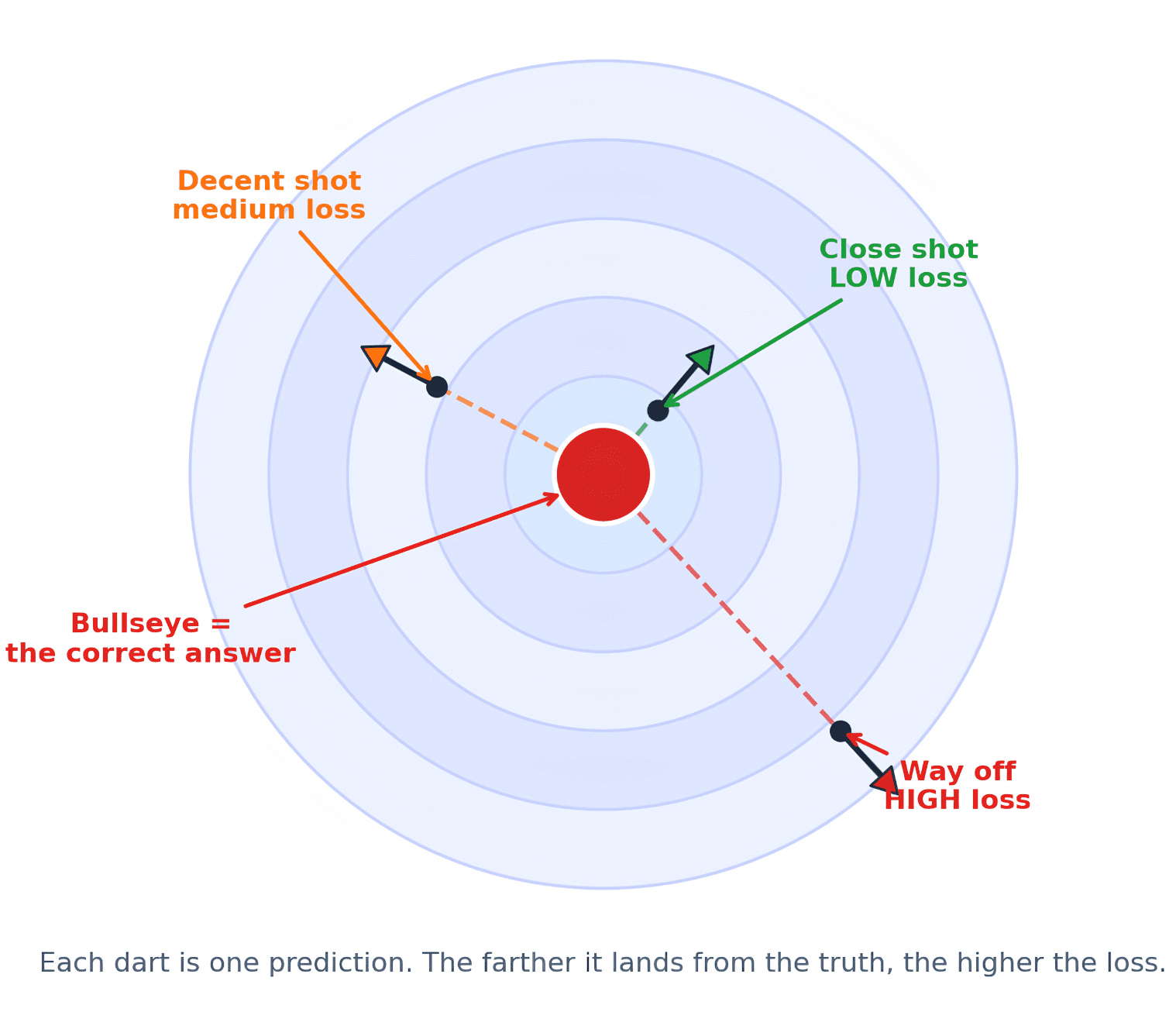
中心からの距離が重要であるのと同様に、中心に近すぎることと、はるかに外れていることは同じではありません。同様に、モデルにとって答えが間違っていることを知るだけでは不十分です。改善するためには、モデルがどれほど失敗したかを理解する必要があります。
損失関数が何であり、なぜそれが必要なのかを理解したので、機械学習でよく使われるいくつかの一般的な損失関数を見てみましょう。**
# 平均二乗誤差 (Mean Squared Error)
**
数を予測するための最も一般的な損失関数は、平均二乗誤差(MSE)です。これは、モデルが家の価格や気温、配送時間などの数を予測する際に頻繁に使用されます。考え方は非常にシンプルです。
- エラー:各予測について、推測と真の値とのギャップを計算します。
- 二乗:各ギャップを自分自身で掛けます(自乗します)。
- 平均:それらすべての二乗されたギャップの平均を取ります。
これを Python で以下のように記述できます:
def mean_squared_error(predictions, actuals):
    squared_errors = [(p - a) ** 2 for p, a in zip(predictions, actuals)]
    return sum(squared_errors) / len(squared_errors)
さて、誤差を計算して予測値全体で平均を取る直感的な意味は理解できるでしょうが、なぜ誤差を二乗するのかについては混乱しやすい点です。これには2つの理由があります:
- 二乗することですべての誤差が正の値になります。+3 の誤差と -3 の誤差はどちらも同様に悪いですが、二乗すると両方とも9になり、互いに相殺されることがなくなります。
- 二乗することで大きなミスを小さなミスよりもはるかに厳しく罰します。これは多くのユースケースで有効です。例えば家賃価格を予測する場合、1,000 ドル間違えることと200,000 ドル間違えることは、それぞれ相応に罰せられるべきです。
# 平均絶対誤差 (Mean Absolute Error)
もう一つの一般的な損失関数として、平均絶対誤差(MAE: Mean Absolute Error)があります。MAE も予測値と実際の値の間のギャップを測定しますが、誤差を二乗しません。代わりに単に絶対値**を取ります。
これを実装する Python 関数は以下の通りです:
def mean_absolute_error(predictions, actuals):
    absolute_errors = [abs(p - a) for p, a in zip(predictions, actuals)]
    return sum(absolute_errors) / len(absolute_errors)
つまり、大きな誤差を罰しますが、MSE(平均二乗誤差)ほど厳しくはありません。
- 10 の誤差はコスト10となり、20 の誤差はコスト20となります。
- データに自然な外れ値が含まれており、モデルが過剰反応しないようにしたい場合、MAE は良い選択肢です。
MSE と MAE の曲線を比較する簡単なグラフを示しましょう。
**

# クロスエントロピー損失 (Cross-Entropy Loss)
これまで、数値の予測について話してきました。しかし、多くの機械学習の問題はカテゴリの予測に関するものです。
このメールはスパムか否か?
これは猫、犬、魚の写真のどちらか?
ある取引は不正行為か否か?
分類タスクでは、モデルは通常以下のような確率を出力します:
犬:70%
猫:20%
魚:10%
もし画像が本当に犬であれば、それは良い予測です。しかし、それが猫である場合、モデルは正解に対して低い確率を割り当てたことでペナルティを受ける必要があります。
したがって、直感的な理解は以下のようになります:
- 正解かつ自信あり — 損失小
- 正解だが自信なし — 損失中
- 誤りかつ自信あり — 損失大
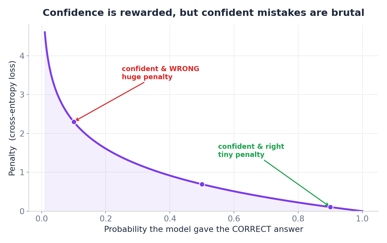
これがクロスエントロピーが分類において広く使用されている理由です。それは単にモデルが正解だったかどうかだけでなく、モデルの自信度合いにも注目します。
# 損失と精度の違い (Loss vs. Accuracy)
異なる損失関数について説明したので、ここで「損失」と「精度」の違いを明確にしておきたいと思います。これらは同じものではありません。
精度 (Accuracy) は どれだけの予測が正しかったか を示します。
一方、損失 (Loss) は モデルの誤りがどれだけ悪かったか を示します。
もしモデル A とモデル B の 2 つのモデルがあり、どちらも 100 回の予測のうち 90 回を正解した場合、両者の精度(accuracy)は同じになります。しかし、一方のモデルは正しい答えに対して非常に自信を持っており、誤った答えに対してもわずかな誤りしかしていない可能性があります。他方のモデルは多くの例で barely 正解しているだけで、間違っている時には極めて高い自信を持っている可能性があります。
その場合、精度は同じでも、損失(loss)は異なります。
# トレーニングループ
**
モデルが損失の数値を持つと、改善が可能になります。トレーニングループは以下のようになります:
- モデルが予測を行います。
- 損失関数が誤りを測定します。
- オプティマイザ(optimizer)がモデルを更新します。
- モデルが再び試みます。
- 損失が hopefully 小さくなることを期待します。
モデルをトレーニングする際、時間経過に伴う損失の推移もプロットします。初期段階では、モデルは多くの誤りを犯し予測が苦手なため、損失は高くなります。しかし、トレーニングが進むにつれて損失は減少し、モデルは予測を行うのが上手になっていきます。
健全なトレーニングカーブ(training curve)は通常、以下のような様子を示します:
初期に高い損失 → 急激な低下 → 徐々に平坦化****
これは以下の図で確認できます。

平坦化は正常です。これはモデルが簡単なパターンを学習し、現在はより小さな改善を行っていることを意味します。しかし、トレーニング損失が低下する一方で検証損失が上昇し始めると、過学習の警告サインとなる可能性があります。つまり、モデルが一般化するパターンを学ぶのではなく、トレーニングデータを暗記しているおそれがあるのです。
# 最後のまとめ
**
損失関数は、モデルの誤りスコアです。
これはモデルに予測がどれほど間違っているかを伝え、学習に対して明確な目標を与えます:その数値を小さくすることです。
損失関数を理解すれば、勾配降下法、逆伝播、最適化、過学習、評価指標など、他の多くの機械学習の概念も理解しやすくなります。
恐ろしい数式から始める必要はありません。次の考えから始めましょう:
- モデルが推測する。
- 損失関数がその推測を採点する。
- モデルはスコアを減らすように自身を更新する。
これが機械学習の核心です。
損失とは、モデルが自分が間違っていると知る方法です。
トレーニングとは、より間違いを少なくする方法を学ぶプロセスです。
これで本記事は終わりです。当シリーズの「初心者向け」では、今後もいくつかの興味深い概念を取り上げていきます。
Kanwal Mehreen は、データサイエンスと AI と医療の交差点に深い情熱を持つ機械学習エンジニアであり技術ライターです。彼女は「ChatGPT で生産性を最大化する」という電子書籍の共著者でもあります。APAC 地域の Google Generation Scholar 2022 に選出され、多様性と学術的卓越性を提唱しています。また、Teradata Diversity in Tech Scholar、Mitacs Globalink Research Scholar、Harvard WeCode Scholar としても認められています。Kanwal は変化の熱心な支持者であり、STEM 分野における女性のエンパワーメントを目的とした FEMCodes を設立しました。
原文を表示
**
# Introduction
I know that when beginners start learning machine learning, things seem easy at first. You follow a tutorial that asks you to load a dataset, train a model, and then you see something like this: loss = "mse" or criterion = nn.CrossEntropyLoss().
And just like that, the tutorial starts talking about equations, gradients, optimization, and Greek letters. If you have ever nodded along without really understanding what a loss function does, you are not alone. Loss functions are often explained backward.** Most tutorials start with the formula when they should start with the idea. This article is part of my noob series, where I will make things easier for you to understand. So, let's get started.
# What Is a Loss Function?
**
A loss function is how a machine learning model knows how wrong it is. That is literally the whole concept. The model makes a prediction. The loss function compares that prediction with the correct answer. Then it gives the model a number that says, "This is how bad your mistake was."
A high loss means the model was very wrong**.
A low loss means the model was close.
During training, the model keeps adjusting itself to make the loss smaller.
That is how learning happens. If you have played a dart game, it is very similar. You throw the dart. To improve, you need feedback. You need to know whether your dart was slightly off, far away, too high, or too far left. Without that feedback, you cannot improve. So, the bullseye is basically the correct answer and the dart is the prediction. You measure the distance between the dart and the bullseye. The loss function measures how far away the dart landed. That distance becomes the model's feedback signal. Here's how it would look if you prefer a visualization.
**
Just like the distance from the center matters, throwing too close is not the same as being way off. Similarly, for models, just knowing that the answer is wrong is not enough. The model needs to know how badly it failed in order to improve.
Now that we have an understanding of what a loss function is and why we need it, let's look at some of the common loss functions used in machine learning**.
# Mean Squared Error
**
The most common loss for predicting numbers is mean squared error (MSE). It is often used when the model is predicting numbers like house prices, temperatures, or delivery times. The idea is very simple.
- Error: For each prediction, take the gap between the guess and the truth.
- Squared: Multiply each gap by itself.
- Mean: Average all those squared gaps.
You can write it in Python like this:
def mean_squared_error(predictions, actuals):
squared_errors = [(p - a) ** 2 for p, a in zip(predictions, actuals)]
return sum(squared_errors) / len(squared_errors)Now, I know that taking the errors and then averaging over the predictions makes sense intuitively, but understanding why we square them can be confusing. This is done for two reasons:
- Squaring makes every error positive. An error of +3 and an error of -3 are equally bad, and squaring turns both into 9, so they stop cancelling each other out.
- Squaring punishes big mistakes far more harshly than small ones. This is good for lots of use cases. For example, if you are predicting house prices, being wrong by \$1,000 versus \$200,000 should be punished accordingly.
# Mean Absolute Error
Another common loss function is mean absolute error (MAE). MAE also measures the gap between predictions and actual values, but it does not square the error. Instead, it simply takes the absolute value**.
Here's the Python function to write it:
def mean_absolute_error(predictions, actuals):
absolute_errors = [abs(p - a) for p, a in zip(predictions, actuals)]
return sum(absolute_errors) / len(absolute_errors)So, it punishes large errors, but not as harshly as MSE does.
- An error of 10 costs 10 and an error of 20 costs 20.
- If your data naturally has some outliers and you do not want your model to overreact, MAE is a good choice.
Let me show a quick graph that compares the MSE and MAE curves.
**
# Cross-Entropy Loss
So far, we have talked about predicting numbers. But many machine learning problems are about predicting categories.
Is this email spam or not?
Is this a picture of a cat, dog, or fish?
Is a certain transaction fraudulent or not?
For classification tasks, models usually output probabilities like:
Dog: 70%
Cat: 20%
Fish: 10%
If the image really is a dog, that is a good prediction. But if it is a cat, then the model needs to be penalized for assigning a lower probability to the correct answer.
So, the intuition is:
- Correct and confident — low loss
- Correct but unsure — medium loss
- Wrong and confident — high loss
This is why cross-entropy is so widely used for classification. It does not just care about whether the model was right. It also cares about how confident the model was.
# Loss vs. Accuracy
Now that we have gone through different loss functions, I also want to clarify the difference between loss and accuracy. They are not the same thing.
Accuracy tells you how many predictions were correct**.
But loss tells you how bad the model's mistakes were.
If you have two models — Model A and Model B — and both get 90 out of 100 predictions correct, they will have the same accuracy. But one model may be very confident on the right answers and only slightly wrong on the incorrect ones, while the other may be barely correct on many examples and extremely confident when wrong.
In that case, the accuracy would be the same, but the loss would be different.
# The Training Loop
**
Once the model has a loss number, it can improve. The training loop looks like this:
- The model makes predictions.
- The loss function measures the mistakes.
- The optimizer updates the model.
- The model tries again.
- The loss hopefully gets smaller.
When training a model, we also plot the loss over time. In the beginning, the model makes many mistakes and is poor at making predictions, so the loss is high. But as training progresses, the loss decreases and the model gets better at making predictions.
A healthy training curve often looks like this:
High loss at the start → sharp drop → gradual flattening****
as you can see in the figure below.
The flattening is normal. It means the model has learned the easy patterns and is now making smaller improvements. But if the training loss goes down while the validation loss starts going up, that can be a warning sign of overfitting** — which means the model may be memorizing the training data instead of learning patterns that generalize.
# Final Thoughts
**
A loss function is the model's mistake score.
It tells the model how wrong its predictions are, and it gives training a clear goal: make that number smaller.
Once you understand loss functions, many other machine learning ideas become easier to grasp — including gradient descent, backpropagation, optimization, overfitting, and evaluation metrics.
You do not need to start with scary equations. Start with the idea:
- The model guesses.
- The loss function scores the guess.
- The model updates itself to reduce the score.
That is the heart of machine learning.
Loss is how a model knows it is wrong.
Training is how it learns to be less wrong.
This brings us to the end of this article. We will continue to cover some interesting concepts throughout our noob series.
Kanwal Mehreen** is a machine learning engineer and a technical writer with a profound passion for data science and the intersection of AI with medicine. She co-authored the ebook "Maximizing Productivity with ChatGPT". As a Google Generation Scholar 2022 for APAC, she champions diversity and academic excellence. She's also recognized as a Teradata Diversity in Tech Scholar, Mitacs Globalink Research Scholar, and Harvard WeCode Scholar. Kanwal is an ardent advocate for change, having founded FEMCodes to empower women in STEM fields.
関連記事
金属合金の挙動をより良くモデル化する新手法
MIT の研究チームが、ロケットや半導体などでの材料挙動予測を困難にする複雑な化学配列をシミュレーションする新たなアプローチを開発し、コストと時間を削減する可能性を示した。
機械学習研究の芸術と禅(11 分読了)
TLDR AI は、AI 研究者になるための道は読み込みと構築にあり、成功には時間と努力、そして世界クラスとなるためには並外れた規律が必要であると述べている。
Python の sktime を用いた時系列機械学習モデルの構築方法
KDnuggets が公開した記事で、Python ライブラリ「sktime」を使用した時系列データ分析と機械学習モデルの作成手法について解説している。
今日のまとめ
AI日報で今日の重要ニュースをまとめ読み