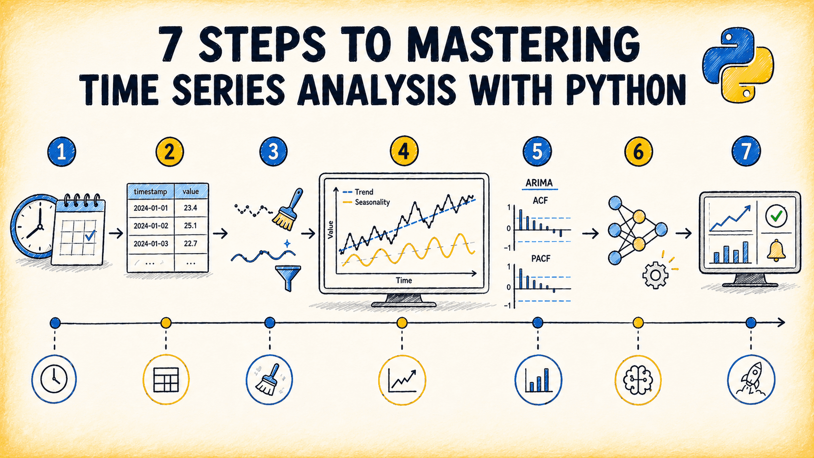
Python を用いた時系列分析の習得に向けた7 つのステップ

**

# Introduction

Time series data is everywhere — energy consumption logged hourly, transactions recorded to the millisecond, patient vitals tracked across hospital stays, inventory levels updated daily, and more. Analyzing, modeling, and forecasting this kind of data is one of the most in-demand skills across industries.

What makes time series distinct from general data science is that it demands a different mental model at every stage. Temporal ordering, autocorrelation, seasonality, and non-stationarity are structural properties that don't exist in tabular data but define everything about how time series behave. The seven steps outlined in this article will help you learn and become proficient in time series analysis with Python.

# Step 1: Understanding What Makes Time Series Data Different

To get started, you need to understand the properties that make time series structurally different from tabular data. Many practitioners skip this step, assuming general machine learning knowledge transfers directly. It doesn't, at least not without adjustment.

The three most important structural properties are summarized below:

Property

What it means

Why it matters

Temporal dependence

Observations are not independent; what happened yesterday correlates with today

Standard machine learning problems assume row independence, so applying it naively produces misleading results

Stationarity

Statistical properties remain constant over time

Most classical models require stationarity; most real-world series lack it and need differencing or transformation

Seasonality and trend

Regular repeating patterns or seasonality combined with long-run directional movement or trend**

Separating these from the irregular residual is often the core analytical challenge

Resource: Rob Hyndman and George Athanasopoulos's free online textbook Forecasting: Principles and Practice (3rd ed.) is a comprehensive reference. If you're interested in learning some serious time series analysis, you may want to bookmark it before proceeding to any modeling step.

# Step 2: Mastering Time Series Data Structures in Python

**

Working with time series in Python means being comfortable with pandas' time-aware data structures: DatetimeIndex, PeriodIndex, resampling, and rolling operations.

The distinction between DatetimeIndex and PeriodIndex** matters more than it first appears.

• DatetimeIndex represents specific moments in time.
• PeriodIndex represents spans of time.

Knowing when to use each, how to convert between them, and how to parse, slice, and resample time-indexed data saves significant friction later, since most modeling libraries have specific format requirements of their own.

Resampling and aggregation is where many analysts make quiet, consequential errors. Downsampling from minute-level to hourly data requires choosing the right aggregation function, and getting it wrong corrupts the analysis. Practicing resampling with multiple aggregation strategies on the same dataset until the logic is intuitive is time well spent.

Rolling and expanding windows — .rolling() and .expanding() — are the pandas primitives for lag features and cumulative statistics. Building rolling means, standard deviations, and lag offsets by hand before relying on library abstractions is important: understanding what these operations do at the index level prevents a whole class of subtle data leakage errors that are notoriously hard to diagnose after the fact.

Resource: Work through the pandas Time Series and Date Functionality guide with a real dataset before proceeding.

# Step 3: Learning to Clean and Prepare Time Series Data

**

Real-world time series arrives with missing timestamps, sensor dropouts, duplicate readings, and outliers. The cleaning decisions made here propagate through everything downstream, and time series cleaning requires different techniques from tabular cleaning because temporal ordering constrains every operation.

A missing timestamp and a NaN at a present timestamp are different problems. The former requires reindexing to a canonical frequency grid** before imputation can locate it. For NaN values, strategy should match gap length and signal type: time-based interpolation for short gaps in continuous signals, forward fill for step-function variables like equipment states, and seasonal decomposition imputation for long gaps in strongly seasonal series.

Outlier detection in time series demands local rather than global thinking:

• Global statistical thresholds can miss anomalies in non-stationary series.
• Rolling Z-scores and IQR bounds over sliding windows help detect values unusual within their local neighborhood.
• For multivariate sensor data, Isolation Forest detects anomalies that may not appear in individual channels but emerge across combined features.

Frequency alignment deserves attention when joining series recorded at different rates — hourly meter readings merged with daily weather data, for instance. The aggregation function matters as much as the join itself, and documenting the downsampling logic is worth the discipline, because the choice affects model inputs in ways that are invisible in the merged output.

Resource: The sktime transformations documentation covers the most common preprocessing transformations with helpful examples.

# Step 4: Developing Intuition Through Exploratory Analysis

**

You cannot model what you haven't understood, and understanding a time series requires structured exploratory analysis before any model is fit. Exploratory data analysis for time series goes well beyond summary statistics.

Decomposition** should be the first step in any serious analysis. Using statsmodels.tsa.seasonal.seasonal_decompose or the more outlier-robust STL decomposition separates a series into trend, seasonal, and residual components, each of which rewards independent examination.

• Is the trend linear or nonlinear?
• Is the seasonal amplitude stable, or does it shift over time?
• Are the residuals roughly white noise, or do they contain structure the decomposition missed?

Autocorrelation analysis is the other essential diagnostic. The autocorrelation function (ACF) and partial autocorrelation function (PACF) plots are the primary tools for understanding temporal dependence:

• A slowly decaying ACF signals non-stationarity.
• Significant spikes at lag 24 in hourly data signal daily seasonality.
• PACF cutoffs suggest autoregressive (AR) order.

Reading these plots fluently is essential for any classical modeling work.

Stationarity testing rounds out the exploratory workflow. The Augmented Dickey-Fuller (ADF) test and Kwiatkowski–Phillips–Schmidt–Shin (KPSS) test provide statistical evidence for or against stationarity, and running both is worthwhile since they test complementary hypotheses. The results inform whether differencing or transformation is needed before modeling begins.

Resource: The statsmodels time series analysis documentation documents the decomposition, ACF/PACF plotting, and stationarity testing functions you will use most frequently.

# Step 5: Building Classical Statistical Forecasting Models

**

Classical statistical models — ARIMA, Exponential Smoothing, and their extensions — should be the first models you build. They are often surprisingly competitive with more complex approaches on clean, well-understood series, and they force engagement with the structure of the data in ways that machine learning models don't.

Exponential Smoothing (ETS)** is the right starting point. ETS models assign exponentially decaying weights to past observations and cover a wide range of behaviors through additive and multiplicative components for trend and seasonality. Fitting a model with statsmodels.tsa.holtwinters.ExponentialSmoothing and examining its components gives immediate intuition about the series' structure.

ARIMA and SARIMA follow naturally. ARIMA models the autocorrelation structure of a stationary series through autoregressive and moving average terms; SARIMA extends this to handle seasonal patterns.

Evaluation discipline matters as much as model choice. Random cross-validation on time series produces optimistic and unreliable estimates; walk-forward validation — train on the past, predict the next window, advance the window — simulates how the model would actually perform in production. TimeSeriesSplit from scikit-learn or sktime's forecasting cross-validation utilities both implement this correctly.

Resource: Forecasting: Principles and Practice, Chapters 7–9 for ETS and ARIMA, and the statsmodels State Space documentation for Python-specific implementation detail.

# Step 6: Progressing to Machine Learning and Deep Learning Models

**

Once solid classical baselines exist, machine learning models allow richer feature sets, handle complex non-linearities, and scale to large collections of series that would be impractical to model individually.

Tree-based models such as LightGBM and XGBoost** produce strong forecasts when given well-engineered lag features, rolling statistics, and calendar variables. They handle non-linearity and feature interactions automatically, but data leakage is the central risk; lags must be constructed strictly from past values relative to the prediction timestamp. sktime's make_reduction wraps scikit-learn regressors as forecasters safely and handles this bookkeeping correctly.

Global models become relevant when the problem involves hundreds or thousands of related time series — store-level sales, device-level sensors, regional energy demand. Training a single global model across all series often outperforms individual per-series models by sharing statistical strength, and NeuralForecast supports this pattern natively.

Deep learning architectures have the strongest track records on benchmark datasets and handle multi-seasonality, covariates, and long-horizon forecasting better than classical models. NeuralForecast implements all of these with a consistent API and proper temporal cross-validation support. The right time to reach for deep learning is after simpler models have plateaued, not before.

Resource: Kaggle M5 Forecasting competition notebooks are a good starting point, and the top solutions cover the full pipeline from feature engineering to ensembling on a real retail forecasting problem and are freely available.

# Step 7: Deploying and Monitoring Forecasting Systems

**

The operational challenges specific to time series are distinct from general machine learning deployment.

Concept drift and distribution shift** are inherent risks rather than edge cases in time series, because the series are non-stationary by nature. Monitoring forecast error metrics on a rolling basis and setting up automated alerts when error rates exceed thresholds is the baseline. Scheduled retraining pipelines are not optional in any production forecasting system.

Forecast storage and versioning require deliberate design. Production forecasting systems generate predictions continuously, and storing forecasts alongside the actuals they predicted — rather than just the final model outputs — makes it possible to compute retrospective accuracy at every horizon and understand exactly where the model degrades over time.

Backtesting as a deployment gate is the discipline that separates experiments from production-ready systems. Before any model goes live, a rigorous backtest should simulate the full deployment window using only data that would have been available at each step. A model that looks good on a held-out test set but fails a proper backtest is not ready.

Resource: Evidently AI's model monitoring guide for machine learning monitoring including data and prediction drift detection.

# Wrapping Up

**

Time series analysis rewards sequential learning more than most data science disciplines.

Step

Why it matters

Core properties of time series data

Without understanding temporal dependence, stationarity, and seasonality, every subsequent decision rests on shaky ground

Pandas time-aware data structures

Correct indexing, resampling, and window operations are prerequisites for every analysis and modeling task

Cleaning and preparation

Errors introduced here propagate silently through the entire pipeline; temporal ordering makes them harder to catch than in tabular cleaning

Exploratory analysis

Decomposition, autocorrelation plots, and stationarity tests reveal the structure that determines which models are appropriate

Classical statistical models

Forces structural engagement with the data; often competitive with complex approaches and always useful as a baseline

Machine learning and deep learning models

Extends capability to non-linear patterns, rich feature sets, and large collections of series once classical baselines are understood

Deployment and monitoring

A model that cannot be maintained in production is not a finished product; time series systems require domain-specific operational discipline

Foundation models for time series** — pre-trained on large corpora of diverse series and fine-tuned for specific tasks — are substantially changing how practitioners approach forecasting. Building strong fundamentals in classical and machine learning-based approaches will certainly be useful going forward.

Bala Priya C is a developer and technical writer from India. She likes working at the intersection of math, programming, data science, and content creation. Her areas of interest and expertise include DevOps, data science, and natural language processing. She enjoys reading, writing, coding, and coffee! Currently, she's working on learning and sharing her knowledge with the developer community by authoring tutorials, how-to guides, opinion pieces, and more. Bala also creates engaging resource overviews and coding tutorials.