Python でゼロからベクトル検索を構築する方法
この記事は、NumPy を使用してゼロからベクトル検索エンジンを構築する手順を解説し、埋め込みの保存やコサイン類似度の計算原理など、機械学習モデルの背後にある数値的仕組みを明確に理解させる実用的なチュートリアルである。
キーポイント
ベクトル検索と従来のキーワード検索の違い
従来のキーワード検索が単語の完全一致を求めるのに対し、ベクトル検索は文脈や意味を数値空間上の点(埋め込み)として表現し、幾何学的な近接性で類似性を判定する。
コサイン類似度の役割と利点
ベクトル間の「近さ」を測る指標としてコサイン類似度が用いられ、単語の絶対的な距離や頻度ではなく、ベクトルの方向性(意味)に焦点を当てることでスケーラビリティを確保する。
NumPy によるゼロからの実装
外部ライブラリに依存せず NumPy のみを用いて、埋め込みの正規化や検索空間の可視化など、ベクトル検索の内部動作を段階的に再現するコード例を提供している。
Simulated Embedding Structure
The tutorial simulates vector embeddings using controlled random data with three distinct semantic clusters (electronics, clothing, furniture) to demonstrate concepts without requiring a real ML model.
Dimensionality Reduction for Clarity
A reduced 8-dimensional space is used instead of high-dimensional vectors to make the clustering and search logic easier to visualize and understand in this tutorial context.
正規化による計算効率化
ベクトルをL2正規化することでコサイン類似度の計算が内積に置き換わり、計算コストを削減できます。
単純な行列演算での検索
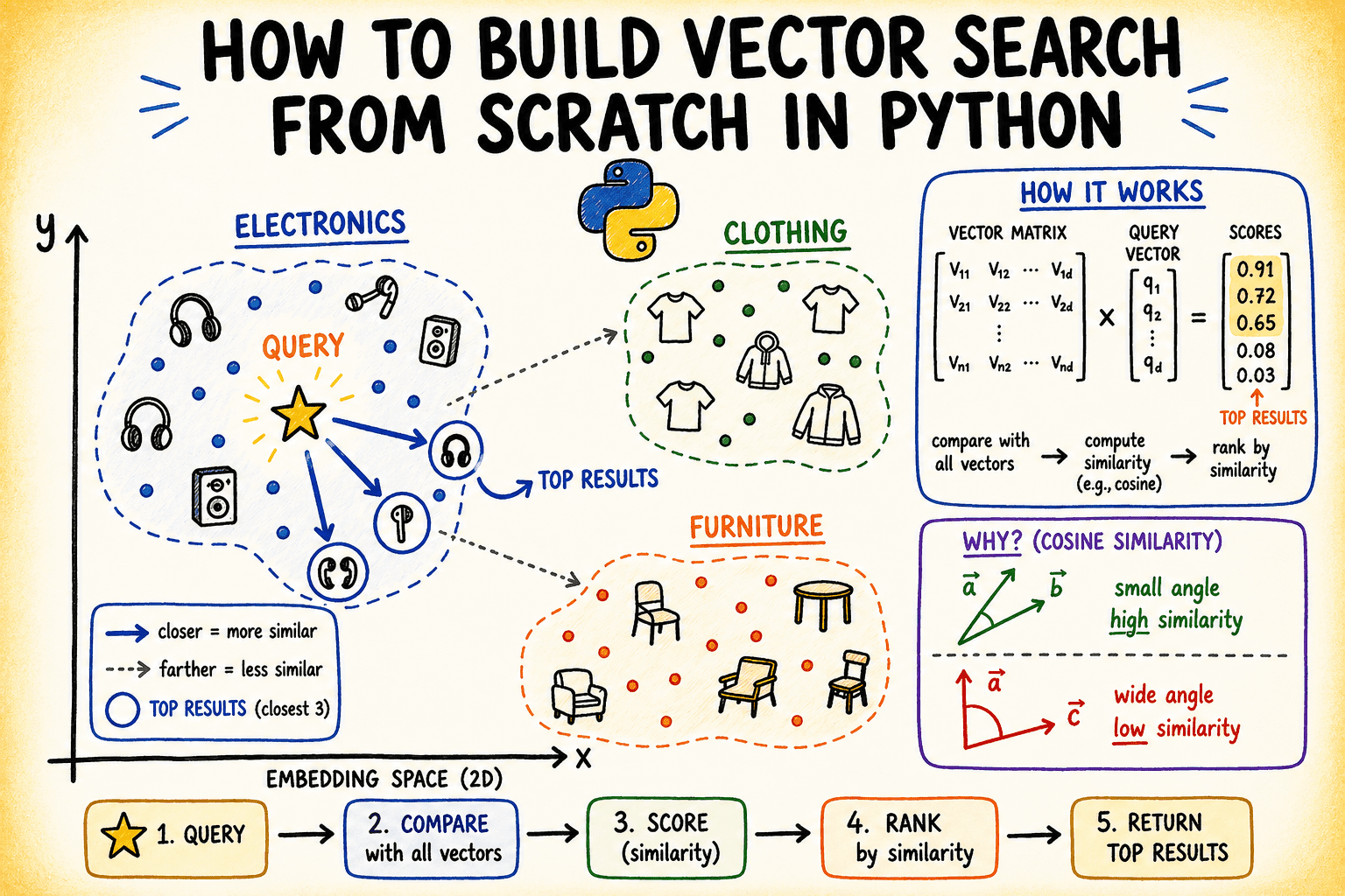
検索処理はクエリの正規化と全ベクトルとの行列乗算(dot product)のみで完結し、その後スコア順にソートして上位k件を返します。
重要な引用
"The gap between 'finding exact words' and 'understanding what someone actually means' is what makes a search feature useful."
"Two sentences can share zero words and still end up neighbors because the model learned that their meanings are close."
"Closeness in vector space means semantic similarity."
In a real system, you'd generate these embeddings from a model like sentence-transformers.
The product names won't be used by the search engine; only the embeddings matter.
"Normalization is important here because it makes cosine similarity equivalent to a dot product, which is cheaper to compute."
影響分析・編集コメントを表示
影響分析
この記事は、ベクトル検索という高度な技術のブラックボックス化が進む中で、その背後にある数学的・計算論的な原理を初学者やエンジニアが再構築する機会を提供します。特に LLM や推薦システムの実装において、既存ライブラリへの依存だけでなく基礎的な理解を深めることで、パフォーマンスチューニングやカスタム実装の基盤となる重要な知見を与えます。
編集コメント
ライブラリに頼りきりの実装が増える中、基礎となる数値計算の仕組みを自らコードで再現する姿勢は、AI エンジニアリングの根幹を固める上で極めて重要です。
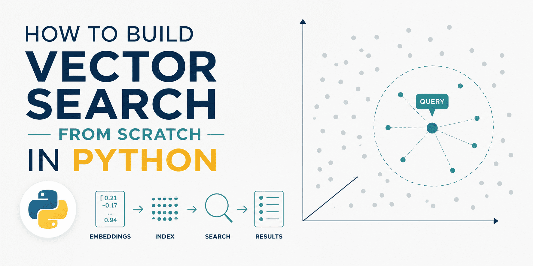
# イントロダクション
**
おそらく、検索バーに質問を入力して、単語は一致するが意味は全く理解されていない結果が表示された経験があるでしょう。あるいは、直接検索していないにもかかわらず、推薦エンジン が驚くほど関連性の高いものを表示しているのを見たことがあるかもしれません。
「正確な単語を見つけること」と「誰かが実際に何を意味しているかを理解すること」の間のギャップこそが、検索機能を*有用なもの*にする要因です。
ベクトル検索 は、テキストを高次元空間内の点として表現することでこのギャップを埋めます。ここで幾何学的な近接性が意味的な類似性を符号化します。2 つの文は単語を共有していなくても、モデルがそれらの意味が近いことを学習しているため、隣り合う位置に配置されることがあります。
この記事では、NumPy だけを使用して Python でゼロからベクトル検索エンジンを構築し、各ステップで何が起こっているかを明確に見ていきます。埋め込み(embeddings)がどのように保存および正規化されるか、なぜコサイン類似度(cosine similarity)が内積(dot product)に還元されるのか、そして 2 次元に投影した際に実際の検索空間がどのようなものになるかについて解説します。
# ベクトル検索とは何か?
従来のキーワード検索 は、単語の完全一致を探します。一方、ベクトル検索は異なるアプローチを取ります:ドキュメントとクエリを数値ベクトルである埋め込み(embeddings)に変換し、高次元空間内で互いに最も近いベクトルを見つけます。
重要な洞察は、ベクトル空間における近さが意味的な類似性を意味することです。同じ意味を持つ 2 つの文—even if they share no words—でも、単語を共有していなくても、埋め込みは互いの近くに位置します。
「近さ」を測定するために使用する距離計測(distance metric)が、システム全体を駆動する鍵となります。最も一般的なのは コサイン類似度 で、これは絶対的な距離ではなく 2 つのベクトル間の角度を測定します。これによりスケーリング不変性(scale-invariant)が実現され、大きさや単語数よりも方向や意味に関心がある場合に有用です。
# データセットの設定
**
架空の e コマースカタログからの短い商品説明のセットを使用します。これらの説明は 8 次元ベクトルとして事前埋め込み済みです—これは概念を実証するのに十分現実的な、大幅に削減された次元数です。
実際のシステムでは、sentence-transformers のようなモデルからこれらの埋め込みを生成します。このチュートリアルでは、明確なクラスター構造を持つ制御されたランダムデータを用いて、そのステップをシミュレーションします。
import numpy as np
np.random.seed(42)
プロダクトカタログ — 3 つのセマンティッククラスタ:電子機器、衣類、家具
products = [
"バッテリー持続時間 30 時間のワイヤレスノイズキャンセリングヘッドフォン",
"防水デザインの Bluetooth スピーカー",
"7 ポート搭載で給電機能付き USB-C ハブ",
"6 フィートの編組 4K HDMI ケーブル",
"RGB バックライト付きメカニカルキーボード",
"メンズスリムフィットチノパンツネイビーブルー",
"レディースメリノウールタートルネックセーター",
"ユニセックスランニングジャケット軽量ウィンドブレーカー",
"メンズレザーチェルシーブーツ",
"オーガニックコットンクルーネック T シャツ",
"6 人掛けソリッドオークダイニングテーブル",
"エルゴノミクスメッシュオフィスチェア腰部サポート付き",
"3 人掛けリネンソファナチュラルベージュ",
"5 段調整式竹製本棚",
"クイーンサイズメモリフォームマットレスミディアムハード",
]
クラスタ構造をシミュレートした埋め込みベクトル生成
8 次元空間におけるクラスタ中心点
electronics_center = np.array([0.9, 0.1, 0.2, 0.8, 0.1, 0.3, 0.7, 0.2])
clothing_center = np.array([0.1, 0.8, 0.7, 0.1, 0.9, 0.2, 0.1, 0.8])
furniture_center = np.array([0.2, 0.3, 0.9, 0.2, 0.1, 0.9, 0.3, 0.1])
クラスタあたりのサンプル数 n_per_cluster = 5
ノイズの大きさ noise = 0.08
embeddings = np.vstack([
electronics_center + np.random.randn(n_per_cluster, 8) * noise,
clothing_center + np.random.randn(n_per_cluster, 8) * noise,
furniture_center + np.random.randn(n_per_cluster, 8) * noise,
])
print(f"埋め込みベクトルの形状:{embeddings.shape}")
出力:
埋め込みベクトルの形状:(15, 8)
各行は製品を表し、各列はその埋め込みの次元の一つです。検索エンジンでは製品名は使用されず、埋め込みのみが重要です。
 image**
画像:著者提供
# インデックスの構築
ベクトル検索エンジンにおける「インデックス」とは、保存された正規化済み埋め込みのセットに過ぎません。ここで正規化が重要なのは、コサイン類似度が内積と等価になるためであり、計算コストが低くなるからです。
def normalize(vectors: np.ndarray) -> np.ndarray:
"""各行ベクトルを L2 正規化する。"""
norms = np.linalg.norm(vectors, axis=1, keepdims=True)
# 0 で割るのを防ぐ
norms = np.where(norms == 0, 1e-10, norms)
return vectors / norms
class VectorIndex:
def __init__(self):
self.vectors = None
self.labels = None
def add(self, vectors: np.ndarray, labels: list):
self.vectors = normalize(vectors)
self.labels = labels
print(f"{len(labels)} 件のアイテムを、{vectors.shape[1]}次元の埋め込みでインデックス化しました。")
def search(self, query_vector: np.ndarray, top_k: int = 3):
query_norm = normalize(query_vector.reshape(1, -1))
# コサイン類似度 = 正規化されたベクトルの内積
scores = self.vectors @ query_norm.T # shape: (n_items, 1)
scores = scores.flatten()
# スコアの降順でソートされた top-k インデックスを取得
top_indices = np.argsort(scores)[::-1][:top_k]
return [(self.labels[i], float(scores[i])) for i in top_indices]
index = VectorIndex()
index.add(embeddings, products)
Output:
Indexed 15 items with 8-dimensional embeddings.
The search method does three things: normalizes the query, computes dot products against every stored vector, then sorts by score and returns the top-k results. That matrix multiplication (self.vectors @ query_norm.T) is the entire retrieval step.
# Running Queries
Now let's test what we've built with a few queries. We construct query vectors by starting from one of the cluster centers and adding a little noise to simulate a real query embedding.
def make_query(center: np.ndarray, noise_scale: float = 0.05) -> np.ndarray:
return center + np.random.randn(8) * noise_scale
queries = {
"audio equipment": make_query(electronics_center),
"casual wear": make_query(clothing_center),
"home furniture": make_query(furniture_center),
}
for query_name, q_vec in queries.items():
print(f"\nQuery: '{query_name}'")
results = index.search(q_vec, top_k=3)
for rank, (label, score) in enumerate(results, 1):
print(f" {rank}. [{score:.4f}] {label}")
Output:
Query: 'audio equipment'
- [0.9856] Wireless noise-cancelling headphones with 30-hour battery
- [0.9840] USB-C hub with 7 ports and power delivery
- [0.9829] Mechanical keyboard with RGB backlight
Query: 'casual wear'
- [0.9960] Men's slim-fit chino pants navy blue
- [0.9958] Leather chelsea boots for men
- [0.9916] Women's merino wool turtleneck sweater
Query: 'home furniture'
- [0.9929] Bamboo bookshelf 5-tier adjustable
- [0.9902] Linen sofa 3-seater natural beige
- [0.9881] Solid oak dining table seats 6
Scores close to 1.0 mean near-identical direction in embedding space, which is exactly what you expect for queries constructed from the same cluster center as their target documents.
# Visualizing the Embedding Space
High-dimensional data is hard to reason about visually. Principal component analysis (PCA) projects the 8-dimensional embeddings down to 2D so we can see the cluster structure. We'll implement a minimal PCA using only NumPy.
The following code computes the 2D PCA projection and plots all product embeddings with labels and cluster colors:
import matplotlib.pyplot as plt
import matplotlib.patches as mpatches
projected = pca_2d(embeddings)
cluster_colors = (
["#4A90D9"] * 5 + # electronics — blue
["#E8734A"] * 5 + # clothing — orange
["#5BAD72"] * 5 # furniture — green
)
cluster_labels = ["Electronics"] * 5 + ["Clothing"] * 5 + ["Furniture"] * 5
fig, ax = plt.subplots(figsize=(6, 4))
ax.scatter(projected[:, 0], projected[:, 1],
c=cluster_colors, s=100, edgecolors="white", linewidths=0.7, zorder=3)
この部分は、クエリベクトルを同じ空間に投影し、重ね合わせてプロットを完成させる処理です:
Plot query projections
q_projected = pca_2d(
np.vstack(list(queries.values())) - embeddings.mean(axis=0)
)
for (qname, _), (qx, qy) in zip(queries.items(), q_projected):
ax.scatter(qx, qy, marker="*", s=200, color="gold",
edgecolors="#333", linewidths=0.6, zorder=4)
ax.annotate(f"⟵ query: {qname}", (qx, qy),
textcoords="offset points", xytext=(6, -8),
fontsize=7, color="#555555", style="italic")
legend_patches = [
mpatches.Patch(color="#4A90D9", label="Electronics"),
mpatches.Patch(color="#E8734A", label="Clothing"),
mpatches.Patch(color="#5BAD72", label="Furniture"),
mpatches.Patch(color="gold", label="Query vectors"),
]
ax.legend(handles=legend_patches, loc="upper left", fontsize=6)
ax.set_title("Vector Search — Embedding Space (PCA projection)", fontsize=10, pad=10)
ax.set_xlabel("PC 1"); ax.set_ylabel("PC 2")
ax.grid(True, linestyle="--", alpha=0.4)
plt.tight_layout()
plt.savefig("embedding_space_queries_only.png", dpi=150)
plt.show()
Output:
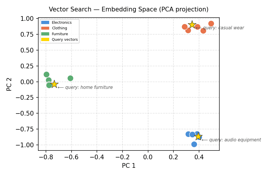
Vector Search — Embedding Space (PCA projection)
The clusters separate cleanly. Each gold star (query vector) lands inside the cluster it was constructed from. This is the geometry that vector search makes use of.
# Visualizing the Similarity Score Distribution
For any given query, it's useful to see how similarity scores are distributed across the whole index — and not just the top-k. This tells you whether the top result is a clear winner or just marginally better than everything else.
q_vec_furniture = queries["home furniture"]
q_norm_furniture = normalize(q_vec_furniture.reshape(1, -1))
all_scores_furniture = (index.vectors @ q_norm_furniture.T).flatten()
sorted_idx_furniture = np.argsort(all_scores_furniture)[::-1]
sorted_scores_furniture = all_scores_furniture[sorted_idx_furniture]
sorted_labels_furniture = [products[i][:30] + "…" if len(products[i]) > 30
else products[i] for i in sorted_idx_furniture]
Define bar colors: green for furniture items, gray for others
bar_colors_furniture = []
for i in sorted_idx_furniture:
if i >= 10 and i <= 14: # Furniture items are originally at indices 10-14
bar_colors_furniture.append("#5BAD72") # Green for furniture
else:
bar_colors_furniture.append("#cccccc") # Gray for others
fig, ax = plt.subplots(figsize=(10, 5))
bars = ax.barh(sorted_labels_furniture[::-1], sorted_scores_furniture[::-1],
color=bar_colors_furniture[::-1], edgecolor="white", height=0.65)
ax.axvline(sorted_scores_furniture[2], color="#5BAD72", linestyle="--",
linewidth=1.2, label="Top-3 cutoff")
ax.set_xlim(sorted_scores_furniture.min() - 0.002, 1.001)
ax.set_xlabel("Cosine Similarity Score")
ax.set_title("Query: 'home furniture' — Similarity Across All Products", fontsize=11, pad=12)
ax.legend(fontsize=8)
ax.grid(axis="x", linestyle="--", alpha=0.4)
plt.tight_layout()
plt.savefig("score_distribution_furniture.png", dpi=150)
plt.show()
Output:
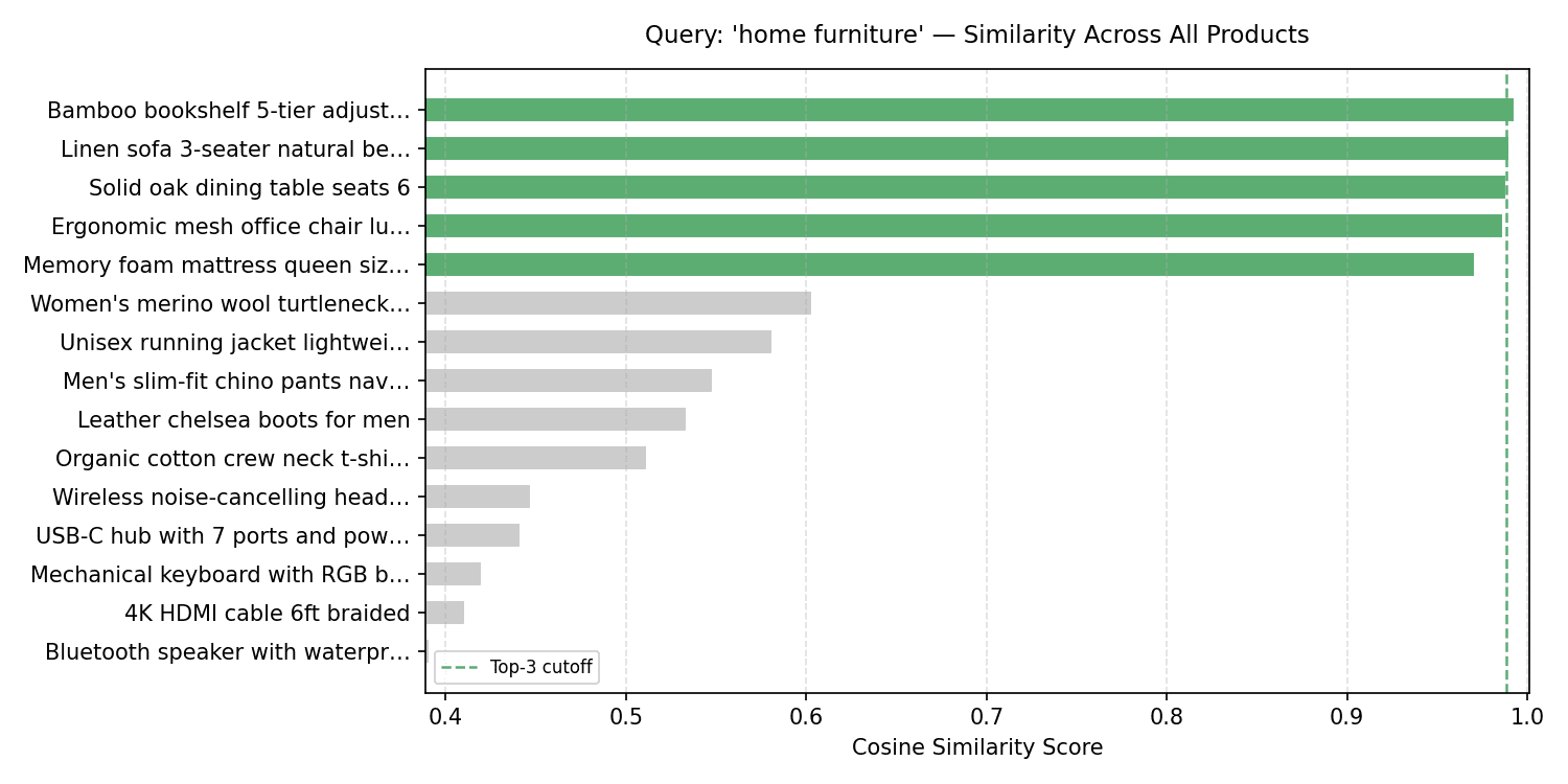
クエリ:'home furniture' — すべての製品間の類似性
家具クラスター(上位 5 つの棒グラフ)とそれ以外の間に明確なギャップが存在します。実際には、このギャップを利用して、結果を完全に抑制する閾値を設定します。
まとめ
あなたは約 50 行の NumPy でベクトル検索エンジンを構築しました。これは、埋め込み表現を正規化して保存するインデックスクラスと、行列乗算を用いてコサイン類似度を計算する検索メソッド、そして結果背後にある幾何学的構造を明らかにする 2 つの可視化から成り立っています。
次のステップは、シミュレーションされた埋め込み表現を実際のものと置き換えることです。sentence-transformers を読み込んで、自分自身のテキストコーパスを埋め込むことを試してみてください。ここで紹介したインデックスコードは、変更なしでそのまま動作します。
さらに「ゼロから始める」シリーズの記事を読みたい場合は、次に見てほしいトピックをお知らせください!
Bala Priya C はインド出身のエンジニア兼技術ライターです。数学、プログラミング、データサイエンス、コンテンツ制作が交差する領域での作業を好んでいます。彼女の専門分野と関心領域には、DevOps、データサイエンス、自然言語処理(NLP)が含まれます。読書、執筆、コーディング、そしてコーヒーを楽しむのが好きです。現在、チュートリアル、ハウツーガイド、意見記事などを執筆することで、開発者コミュニティに知識を共有し、学びを広げる活動を行っています。また、魅力的なリソースの概要やコーディングチュートリアルも作成しています。
原文を表示
# Introduction
**
You've probably typed a question into a search bar and gotten results that matched your words but completely missed your meaning. Or watched a recommendation engine surface something eerily relevant even though you never searched for it directly. The gap between "finding exact words" and "understanding what someone actually means" is what makes a search feature *useful*.
Vector search closes that gap by representing text as points in high-dimensional space, where geometric proximity encodes semantic similarity. Two sentences can share zero words and still end up neighbors because the model learned that their meanings are close.
This article builds a vector search engine from scratch in Python using only NumPy**, so you can see exactly what happens at each step: how embeddings get stored and normalized, why cosine similarity reduces to a dot product, and what the resulting search space actually looks like when you project it down to two dimensions.
You can get the code on GitHub.
# What Is Vector Search?
**
Traditional keyword search looks for exact word matches. Vector search works differently: it converts documents and queries into numerical vectors called embeddings, then finds the vectors that are closest to each other in high-dimensional space.
The key insight is that closeness in vector space means semantic similarity**. Two sentences that mean the same thing — even if they share no words — will have embeddings that are near each other.
The distance metric you use to measure "closeness" is what drives the whole system. The most common one is cosine similarity, which measures the angle between two vectors rather than their absolute distance. This makes it scale-invariant — useful when you care about direction or meaning rather than magnitude or word count.
# Setting Up the Dataset
**
We'll work with a set of short product descriptions from a fictional e-commerce catalog. These are pre-embedded as 8-dimensional vectors — a much reduced dimensionality that is realistic enough to demonstrate the concepts.
In a real system, you'd generate these embeddings from a model like sentence-transformers**. For this tutorial, we simulate that step with controlled random data that has a clear cluster structure.
import numpy as np

np.random.seed(42)

# Product catalog — 3 semantic clusters: electronics, clothing, furniture
products = [
    "Wireless noise-cancelling headphones with 30-hour battery",
    "Bluetooth speaker with waterproof design",
    "USB-C hub with 7 ports and power delivery",
    "4K HDMI cable 6ft braided",
    "Mechanical keyboard with RGB backlight",
    "Men's slim-fit chino pants navy blue",
    "Women's merino wool turtleneck sweater",
    "Unisex running jacket lightweight windbreaker",
    "Leather chelsea boots for men",
    "Organic cotton crew neck t-shirt",
    "Solid oak dining table seats 6",
    "Ergonomic mesh office chair lumbar support",
    "Linen sofa 3-seater natural beige",
    "Bamboo bookshelf 5-tier adjustable",
    "Memory foam mattress queen size medium firm",
]

# Simulate embeddings with cluster structure
# Cluster centers in 8D space
electronics_center = np.array([0.9, 0.1, 0.2, 0.8, 0.1, 0.3, 0.7, 0.2])
clothing_center    = np.array([0.1, 0.8, 0.7, 0.1, 0.9, 0.2, 0.1, 0.8])
furniture_center   = np.array([0.2, 0.3, 0.9, 0.2, 0.1, 0.9, 0.3, 0.1])

n_per_cluster = 5
noise = 0.08

embeddings = np.vstack([
    electronics_center + np.random.randn(n_per_cluster, 8) * noise,
    clothing_center    + np.random.randn(n_per_cluster, 8) * noise,
    furniture_center   + np.random.randn(n_per_cluster, 8) * noise,
])

print(f"Embeddings shape: {embeddings.shape}")
Output:
Embeddings shape: (15, 8)Each row is a product. Each column is one dimension of its embedding. The product names won't be used by the search engine; only the embeddings matter.
**
Image by Author
# Building the Index
The "index" in a vector search engine is just the stored set of normalized embeddings. Normalization is important here because it makes cosine similarity equivalent to a dot product, which is cheaper to compute.
def normalize(vectors: np.ndarray) -> np.ndarray:
    """L2-normalize each row vector."""
    norms = np.linalg.norm(vectors, axis=1, keepdims=True)
    # Avoid division by zero
    norms = np.where(norms == 0, 1e-10, norms)
    return vectors / norms

class VectorIndex:
    def __init__(self):
        self.vectors = None
        self.labels = None

    def add(self, vectors: np.ndarray, labels: list):
        self.vectors = normalize(vectors)
        self.labels = labels
        print(f"Indexed {len(labels)} items with {vectors.shape[1]}-dimensional embeddings.")

    def search(self, query_vector: np.ndarray, top_k: int = 3):
        query_norm = normalize(query_vector.reshape(1, -1))
        # Cosine similarity = dot product of normalized vectors
        scores = self.vectors @ query_norm.T  # shape: (n_items, 1)
        scores = scores.flatten()
        # Get top-k indices sorted by descending score
        top_indices = np.argsort(scores)[::-1][:top_k]
        return [(self.labels[i], float(scores[i])) for i in top_indices]

index = VectorIndex()
index.add(embeddings, products)
Output:
Indexed 15 items with 8-dimensional embeddings.The search method does three things: normalizes the query, computes dot products against every stored vector, then sorts by score and returns the top-k results. That matrix multiplication (self.vectors @ query_norm.T) is the entire retrieval step.
# Running Queries
Now let's test what we've built with a few queries. We construct query vectors by starting from one of the cluster centers and adding a little noise to simulate a real query embedding.
def make_query(center: np.ndarray, noise_scale: float = 0.05) -> np.ndarray:
    return center + np.random.randn(8) * noise_scale

queries = {
    "audio equipment": make_query(electronics_center),
    "casual wear":     make_query(clothing_center),
    "home furniture":  make_query(furniture_center),
}

for query_name, q_vec in queries.items():
    print(f"\nQuery: '{query_name}'")
    results = index.search(q_vec, top_k=3)
    for rank, (label, score) in enumerate(results, 1):
        print(f"  {rank}. [{score:.4f}] {label}")
Output:
Query: 'audio equipment'
  1. [0.9856] Wireless noise-cancelling headphones with 30-hour battery
  2. [0.9840] USB-C hub with 7 ports and power delivery
  3. [0.9829] Mechanical keyboard with RGB backlight

Query: 'casual wear'
  1. [0.9960] Men's slim-fit chino pants navy blue
  2. [0.9958] Leather chelsea boots for men
  3. [0.9916] Women's merino wool turtleneck sweater

Query: 'home furniture'
  1. [0.9929] Bamboo bookshelf 5-tier adjustable
  2. [0.9902] Linen sofa 3-seater natural beige
  3. [0.9881] Solid oak dining table seats 6
Scores close to 1.0 mean near-identical direction in embedding space, which is exactly what you expect for queries constructed from the same cluster center as their target documents.
# Visualizing the Embedding Space
High-dimensional data is hard to reason about visually. Principal component analysis (PCA) projects the 8-dimensional embeddings down to 2D so we can see the cluster structure. We'll implement a minimal PCA using only NumPy.
The following code computes the 2D PCA projection and plots all product embeddings with labels and cluster colors:
import matplotlib.pyplot as plt
import matplotlib.patches as mpatches

projected = pca_2d(embeddings)

cluster_colors = (
    ["#4A90D9"] * 5 +   # electronics — blue
    ["#E8734A"] * 5 +   # clothing — orange
    ["#5BAD72"] * 5     # furniture — green
)
cluster_labels = ["Electronics"] * 5 + ["Clothing"] * 5 + ["Furniture"] * 5

fig, ax = plt.subplots(figsize=(6, 4))
ax.scatter(projected[:, 0], projected[:, 1],
           c=cluster_colors, s=100, edgecolors="white", linewidths=0.7, zorder=3)
This part projects query vectors into the same space, overlays them, and finalizes the plot:
# Plot query projections
q_projected = pca_2d(
    np.vstack(list(queries.values())) - embeddings.mean(axis=0)
)
for (qname, _), (qx, qy) in zip(queries.items(), q_projected):
    ax.scatter(qx, qy, marker="*", s=200, color="gold",
               edgecolors="#333", linewidths=0.6, zorder=4)
    ax.annotate(f"⟵ query: {qname}", (qx, qy),
                textcoords="offset points", xytext=(6, -8),
                fontsize=7, color="#555555", style="italic")

legend_patches = [
    mpatches.Patch(color="#4A90D9", label="Electronics"),
    mpatches.Patch(color="#E8734A", label="Clothing"),
    mpatches.Patch(color="#5BAD72", label="Furniture"),
    mpatches.Patch(color="gold",    label="Query vectors"),
]
ax.legend(handles=legend_patches, loc="upper left", fontsize=6)
ax.set_title("Vector Search — Embedding Space (PCA projection)", fontsize=10, pad=10)
ax.set_xlabel("PC 1"); ax.set_ylabel("PC 2")
ax.grid(True, linestyle="--", alpha=0.4)
plt.tight_layout()
plt.savefig("embedding_space_queries_only.png", dpi=150)
plt.show()
Output:
Vector Search — Embedding Space (PCA projection)
The clusters separate cleanly. Each gold star (query vector) lands inside the cluster it was constructed from. This is the geometry that vector search makes use of.
# Visualizing the Similarity Score Distribution
For any given query, it's useful to see how similarity scores are distributed across the whole index — and not just the top-k. This tells you whether the top result is a clear winner or just marginally better than everything else.
q_vec_furniture = queries["home furniture"]
q_norm_furniture = normalize(q_vec_furniture.reshape(1, -1))
all_scores_furniture = (index.vectors @ q_norm_furniture.T).flatten()

sorted_idx_furniture = np.argsort(all_scores_furniture)[::-1]
sorted_scores_furniture = all_scores_furniture[sorted_idx_furniture]
sorted_labels_furniture = [products[i][:30] + "…" if len(products[i]) > 30
                           else products[i] for i in sorted_idx_furniture]

# Define bar colors: green for furniture items, gray for others
bar_colors_furniture = []
for i in sorted_idx_furniture:
    if i >= 10 and i <= 14:  # Furniture items are originally at indices 10-14
        bar_colors_furniture.append("#5BAD72") # Green for furniture
    else:
        bar_colors_furniture.append("#cccccc") # Gray for others

fig, ax = plt.subplots(figsize=(10, 5))
bars = ax.barh(sorted_labels_furniture[::-1], sorted_scores_furniture[::-1],
               color=bar_colors_furniture[::-1], edgecolor="white", height=0.65)

ax.axvline(sorted_scores_furniture[2], color="#5BAD72", linestyle="--",
           linewidth=1.2, label="Top-3 cutoff")
ax.set_xlim(sorted_scores_furniture.min() - 0.002, 1.001)
ax.set_xlabel("Cosine Similarity Score")
ax.set_title("Query: 'home furniture' — Similarity Across All Products", fontsize=11, pad=12)
ax.legend(fontsize=8)
ax.grid(axis="x", linestyle="--", alpha=0.4)
plt.tight_layout()
plt.savefig("score_distribution_furniture.png", dpi=150)
plt.show()
Output:
Query: 'home furniture' — Similarity Across All Products
There's a visible gap between the furniture cluster (top 5 bars) and everything else. In practice, you'd use this gap to set a similarity threshold below which results are suppressed entirely.
# Wrapping Up
You built a vector search engine with about 50 lines of NumPy: an index class that normalizes and stores embeddings, a search method that uses matrix multiplication to compute cosine similarity, and two visualizations that reveal the geometry behind the results.
The next step is to replace the simulated embeddings with real ones. Try loading sentence-transformers and embedding your own text corpus. The index code here will work without any changes.
If you'd like to read more "from scratch" articles, let us know what you'd like to see next!
Bala Priya C** is a developer and technical writer from India. She likes working at the intersection of math, programming, data science, and content creation. Her areas of interest and expertise include DevOps, data science, and natural language processing. She enjoys reading, writing, coding, and coffee! Currently, she's working on learning and sharing her knowledge with the developer community by authoring tutorials, how-to guides, opinion pieces, and more. Bala also creates engaging resource overviews and coding tutorials.
関連記事
今日のまとめ
AI日報で今日の重要ニュースをまとめ読み