Anyscale、Ray Serve で非同期推論を活用した動画インデックス化サービスの構築事例を公開
本文の状態
日本語全文を表示中
詳細モードで約16分の本文を読めます。
同じ出来事の情報源
この情報源を基点に整理
Anyscale Engineering
Anyscale Engineering は、Ray Serve の非同期推論機能を実装した動画インデックス化サービスの実践例と、高負荷下でのベンチマーク結果を公開し、長時間処理におけるシステム信頼性の向上手法を示した。
AI深層分析を開く2026年8月19日 09:43
AI深層分析
キーポイント
非同期推論の課題解決メカニズム
数秒から数分かかるモデル呼び出しにおいて、リクエスト経路から計算を分離し、メッセージキューと自動スケール機能により、クライアントタイムアウトや接続切断の問題を解消する。
動画インデックス化パイプラインの実装
Anyscale Engineering は非同期推論の概念を実際のサービスとして構築し、長時間かかる処理(動画インデックス化)をバックグラウンドで実行する具体的なアーキテクチャを示した。
高負荷下でのベンチマーク比較
同社は構築したサービスを過酷な負荷条件下でテストし、一般的なマネージドソリューションと比較することで、非同期推論の性能と信頼性の優位性を実証した。
非同期推論のアーキテクチャ構成
Ray Serve は@task_consumer や TaskProcessorConfig を提供し、バックグラウンドでキューから作業を引き継ぐ仕組みを構築する。
動画インデックスサービスの具体的な実装
このサービスは S3 URI を受け取って即座にタスク ID を返し、背景で動画のダウンロード、フレーム分割、SigLIP による埋め込みを行いベクトルを保存する。
重要な引用
Async inference solves these problems by decoupling the request scheduling from the actual computation.
The client submits a job and gets an id back right away, the work goes onto a message queue, a pool of workers, autoscaled to the queue depth, processes it in the background, and the client polls for the result.
"Video indexing is a natural fit for async inference. As each request demands a whole video to download, decode, and embed,it can take seconds to minutes of work..."
"The application, comprises of three deployments, each scaling on its own signal:"
編集コメントを表示
編集コメント
長時間処理を要する AI アプリケーションの開発において、同期処理の限界と非同期処理の利点を具体的に示した有益な技術記事である。実運用での負荷テスト結果が含まれているため、システム設計の参考として価値が高い。
Source Article
元記事を日本語で読む
本文に関係しない購読案内、埋め込み通知、サイト内プロモーションは除いています。
以前の記事で、Ray Serve の非同期推論について紹介しました。これは、メッセージキューを介して長時間実行されるモデル呼び出しをリクエストパスから外し、自動リトライとキュー深度に応じたオートスケーリングをサポートする仕組みです。本稿では、この機能を実際のサービスに適用した事例として、動画インデックス処理パイプラインを構築し、高負荷下で動作させた結果を、一般的なマネージド型ソリューションと比較して解説します。
非同期推論の目的:簡単な復習
機械学習モデルの提供において、音声の文字起こし(1時間分)、動画のインデックス作成、画像や動画の生成など、数秒から数分にわたって実行される単一のモデル呼び出しを行うアプリケーションがあります。通常の同期 HTTP エンドポイントでは、計算が完了するまでリクエスト接続は開かれたままになります。ミリ秒レベルの遅延であればこの結合による影響は見えませんが、このような長時間の処理においては、2 つの重大な問題が発生します。
第一に、数秒から数分かかるリクエストに対してトラフィックが急増すると、ワーカーが処理しきれずに後れを取り、クライアントや中間ノードでタイムアウトが発生します。第二に、数分間接続を保持し続けることは、パケットの損失やホップの失敗に対する暴露時間が増えることを意味します。その結果、予測不能なタイミングでサービスの信頼性やシステム全体の安定性が低下してしまうのです。
非同期推論は、リクエストスケジューリングと実際の計算処理を分離することでこれらの課題を解決します。クライアントはジョブを送信すると即座に ID を受け取り、作業はメッセージキューに格納されます。その後、キューの深さに応じて自動スケーリングされるワーカープールがバックグラウンドで処理を行い、クライアントはその結果をポーリングして取得します。
API と設計については以前の投稿で解説しましたので、ここではその上にサービスを実装し、実世界のトラフィック下でのベンチマークに焦点を当てます。Ray Serve が提供する主な機能は以下の通りです。
「@task_consumer」や「@task_handler」といったデコレータは、デプロイメントメソッドをバックグラウンドワーカーに変換し、キューからタスクを引き受けるようにします。
また、「TaskProcessorConfig」は、実行するメッセージブローカーに対してコードの場所を指示するための設定です(例:) (原文の技術表記: @task_consumer / @task_handler)
Redis や RabbitMQ に対応し、少なくとも一度の配信を保証する仕組み、リトライ機能、デッドレター ルーティングを追加します。
enqueue_task_sync(...)- プロデューサー側から作業をキューに追加し、タスク ID を返す関数です。クライアントはこの ID を使って結果のポーリングを行います。
「AsyncInferenceAutoscalingPolicy」は、キューの深さ(queue depth)に基づいてワーカープールを自動スケールするポリシーです。
LinkThe application: a video-indexing service
非同期推論は、動画インデックス作成サービスのようなユースケースに自然と適合します。各リクエストでは動画のダウンロード、デコード、埋め込み処理が必要となり、数秒から数分かかることが珍しくありません。また、バッチアップロードや夜間のバックフィルなど、トラフィックが突発的に集中する傾向があります。
本サービスの仕組みは以下の通りです。S3 URI を受け取ると即座にタスク ID を返却し、背景では非同期で動画のダウンロード、ffmpeg によるフレーム分割、GPU 上での SigLIP による埋め込み処理、そしてベクトルの S3 への書き出しが行われます。このパイプラインは、1 リクエストあたり数十分を要することもあります。
本アプリケーションは、それぞれが独自のスケール指標に基づいて独立してスケーリングする 3 つのデプロイメントで構成されています。
- IndexingIngress (CPU) - このデプロイメントは
POST /indexエンドポイントを受け付け、ユーザーから送信されたタスクをキューに追加し、タスク ID を返却します。 - VideoIndexConsumer (CPU) -
@task_consumerデコレータを持つこのコンシューマーは、キューからタスクを取り込み、ffmpeg で動画をダウンロードしてチャンク化し、その後エンコーダーを呼び出します。これはキューの深さに応じて自動スケーリングを行うデプロイメントです。 - VideoEncoder (GPU) - SigLIP 神経ネットワークを保持する標準的なデプロイメントです。動画インデックスコンシューマーはハンドルを通じてこれを呼び出すため、フレーム間のデータ移動はネットワーク経由ではなく Ray の RPC を介して行われ、GPU 負荷に応じて独立してスケーリングします。
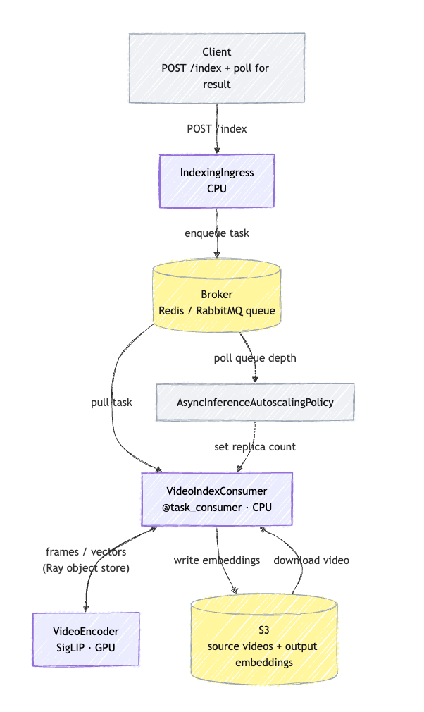
図は、実際に展開・検証したサービスのアーキテクチャを示しています。紫色のボックスがデプロイメントを表し、黄色のボックスがサービスと通信する外部システムを表します。
*展開・検証したサービスのアーキテクチャ*
プロデューサー(ユーザーのリクエストを受け付けるデプロイメント)は非常にシンプルなイングレスデプロイメントです。タスクをキューに追加して ID を返すだけで、呼び出し元が処理完了を待つことはありません。
@serve.ingress(fastapi_app)
class IndexingIngress:
    def __init__(self, consumer):
        self.adapter = instantiate_adapter_from_config(PROCESSOR_CONFIG)

    @fastapi_app.post("/index")
    async def index(self, req: IndexRequest):
        result = self.adapter.enqueue_task_sync(
            task_name=TASK_INDEX_VIDEO,
            kwargs={"video_uri": req.video_uri, "video_id": req.video_id},
        )
        return {"task_id": result.id, "status": result.status}
ビデオインデックスコンシューマーは、単純な同期 Python コードです。ビデオ ID に対して冪等性を保ちながら、CPU で動画をチャンク化し、ハンドルを通じて GPU エンコーダーを呼び出し、結果を保存します。
@serve.deployment(ray_actor_options={"num_cpus": FFMPEG_THREADS}, ...)
@task_consumer(task_processor_config=PROCESSOR_CONFIG)
class VideoIndexConsumer:
    def __init__(self, encoder):
        self.encoder = encoder               # GPU DeploymentHandle

    @task_handler(name=TASK_INDEX_VIDEO)
    def index_video(self, video_uri, video_id=None):
        if is_done(video_id):                  # idempotent on redelivery
            return {"status": "skipped_already_indexed"}
        chunks = chunk_video(download(video_uri))         # CPU: ffmpeg
        refs = [self.encoder.remote(c.frames) for c in chunks]
        vectors = [r.result()["frame_embeddings"] for r in refs]
        write_video_embeddings(video_id, vectors)         # store to S3
        mark_done(video_id)
        return {"status": "indexed", "num_chunks": len(chunks)}
注記 - 以下のベンチマークでは、VideoIndexConsumer(CPU)と VideoEncoder(GPU)のデプロイメントを単一の GPU ワーカーに統合しました。一方で、前面には引き続き軽量なイングレスを維持しています。これは比較を公平にするためであり、また代替手段である Amazon SageMaker がサポートする展開モデルにより近づけるための措置です。
SageMaker では、1 つのエンドポイント背後に CPU サービスと GPU サービスを別々にデプロイすることはできません。唯一の代替手段は、これらを完全に独立したエンドポイントとして公開することですが、この方法では SageMaker はさらに不利になります。中間テンソルが 2 つのエンドポイント間をネットワーク経由で値渡しされる必要がある一方、Ray Serve では共有オブジェクトストアを通じて参照渡しを行うためです。したがって、以下に示すすべてのベンチマーク結果は、前述の 3 デプロイ構成ではなく、イングレスと 1 つの融合ワーカーからなる 2 デプロイ構成で収集したものです。
LinkBehavior under load
今回の目的は、サービスに対する負荷テストを行い、持続的な過負荷下での信頼性とパフォーマンスを評価することです。理想的には、サービスは流入するトラフィックに合わせてスケーリングし、可能な限り迅速にリクエストを処理しながら、ユーザーのリクエストをドロップすることなく動作する必要があります。
信頼性は、負荷テスト中に失敗したリクエスト数を測定することで評価します。一方、パフォーマンスは、システムが負荷の増加に対してどのように応答するか、特にトラフィックに応じてスケーリングアップ・ダウンを行いながらスループットと安定性を維持できる能力を観察することで評価します。
両方の側面を検証するため、持続的な負荷テストとして 20 分間にわたり、通常時 50 RPS(1 秒間あたりのリクエスト数)で、定期的に 100 RPS にスパイクする洪水テストを実施しました。このワークロードは、4 GPU フリートが処理できる能力の約 5〜10 倍に相当し、テスト期間中に約 67,000 の動画リクエストが発生します。
入力されるリクエストレートがフリートの処理能力を大幅に上回るため、リクエストのバックログ(待機列)が生じるのは避けられません。これは、システムが持続的な圧力下でどのようにスケーリングし、耐性を発揮するかを検証する絶好のテストケースです。
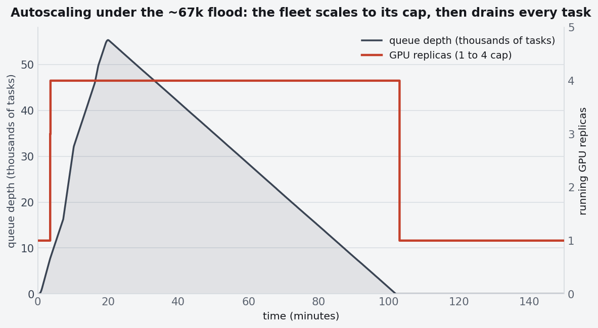
その結果、以下のことが確認できました。
- 需要に応じたレプリカの自動スケーリング - バックログが増加するにつれ、アプリケーションは GPU レプリカ数を自動的に 1 から設定上限の 4 に増やしました。バックログが解消されると、再び 1 に縮小します。固定されたフリート規模はなく、バーストごとに手動チューニングを行う必要もありませんでした。
- 失敗したリクエストゼロ - 約 67,000 の動画リクエストすべてが正常に受け入れられ、キューに入れられ、最終的に処理されました。デッドレターキュー(処理不能なリクエストを格納する場所)はテストを通じて空のままであり、持続的な過負荷下でもリクエストがドロップされたり失敗したりすることはなかったことを示しています。
リンク比較:管理型代替案としての Amazon SageMaker
これらの数値を文脈化するために、同様のワークロードを **Amazon SageMaker Async Inference** で実行しました。これはこの種のワークロードで一般的な管理型ソリューションです。私たちのセットアップと同様に、SageMaker は着信リクエストをキューに積み、バックログに応じてスケーリングし、S3 からの読み書きを行います。
両方の環境では、同じハードウェア(4× NVIDIA T4 GPU)、同じ 1 フレームの SigLIP ワークロード、そして同じ 20 分間の洪水テストを使用しました。どちらも単一のコールドインスタンスから開始しています。SageMaker の非同期エンドポイントが単一のモデルコンテナを実行するのに対し、Ray Serve 側でも上記のように、単一の融合デプロイメントを使用しました。
つまり、両者のデプロイアーキテクチャ、ハードウェア、ワークロードは同一であり、2 つのシステムにおける主要な違いはオーケストレーションエンジンにあります。
| メトリクス(同じ洪水、4x T4) | Ray Serve 非同期 | SageMaker 非同期 |
|---|---|---|
| フルファームへの到達時間(コールド) | ~155 秒 | ~589 秒 |
| アイドル容量の解放(最速測定値) | ~5 秒 | ~104 秒 |
| 自動スケーリング設定 | 1 つのポリシーブロック | 2 つのステップポリシー + 2 つのアラーム(以下で説明)* |
| 失敗/消失したタスク | 0 | 0 |
| ACK レイテンシ、p50(負荷下) | 12.8 ms | 11.8 ms |
SageMaker エンドポイントには、2 つの Application Auto Scaling ステップポリシーを適用して自動スケーリングを行いました。それぞれのポリシーは CloudWatch アラームに紐付けられています。
「バックログ急増」アラームは、1 台あたりの近似バックログサイズが 60 秒間のデータポイントで 5 以上になったときに発火し、「高速アウト」ポリシーをトリガーしてインスタンス数を即座に最大 4 台まで拡張します。一方、「バックログ解消」アラームは、総近似バックログサイズが 1 を下回ったときに発火し、「高速イン」ポリシーをトリガーしてインスタンス数を 1 台まで縮小します。
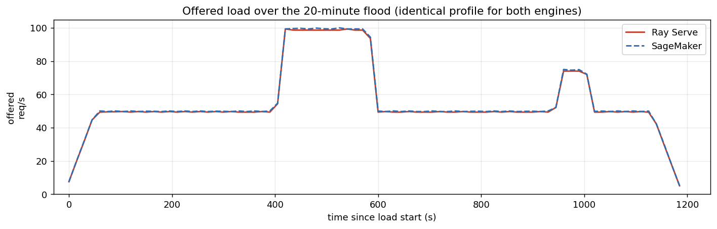
図 1: 時間経過に伴う提供 RPS(両エンジンで同一のプロファイル)
*Offered load over the 20-minute flood (identical profile for both engines)*
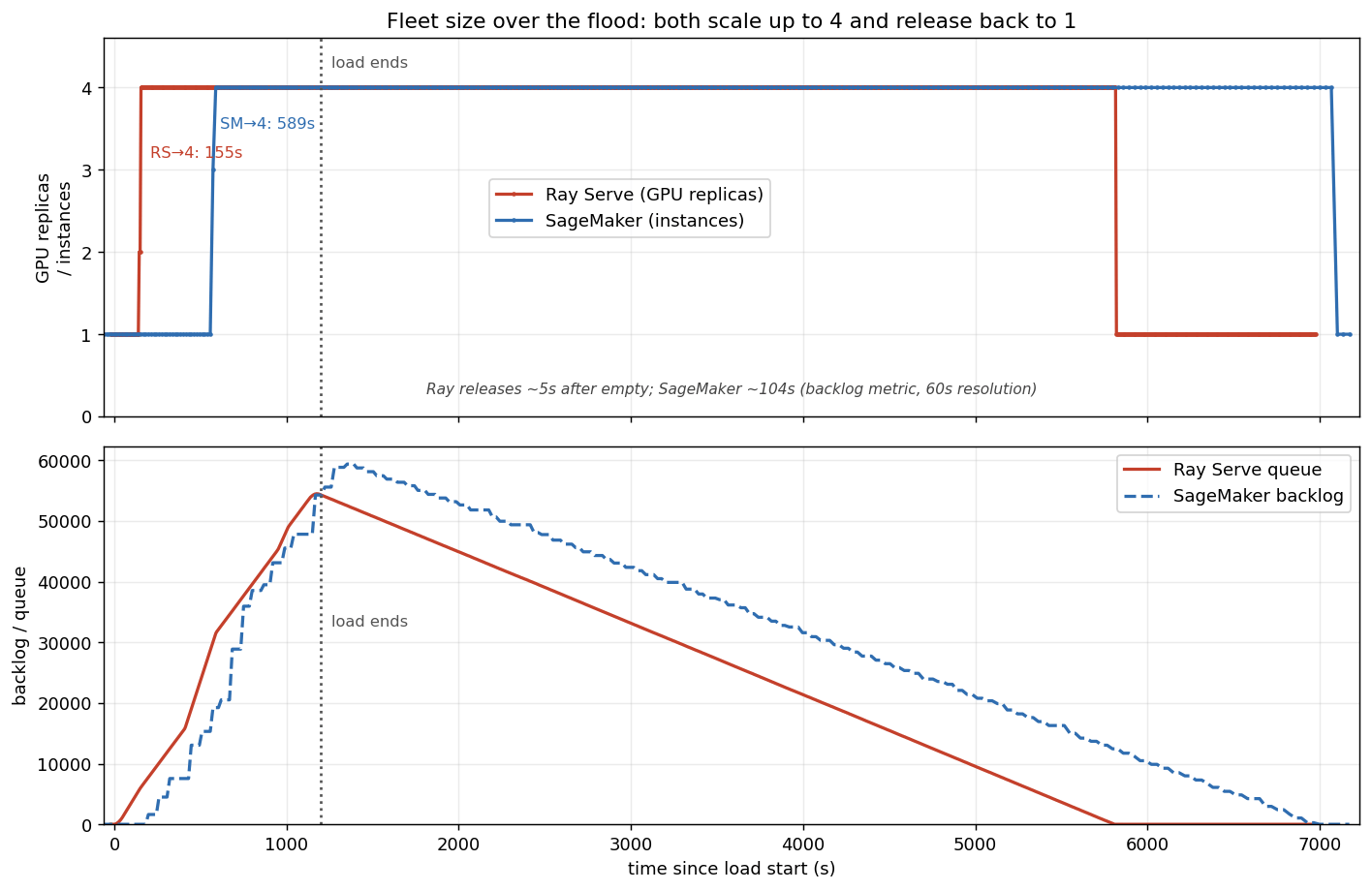
図 1: 時間経過に伴う GPU レプリカ/インスタンス数
図 2: Ray Serve と Amazon SageMaker のバックログキュー長を比較したグラフ
*Fleet size over the flood, both scale up to 4 and release back to 1*
上記の実行結果から、以下の観察点が得られました。
スケーリングの速度はほぼ同等です。両方とも 4 GPU のフルファームに到達するまでの所要時間は同程度で、その大部分がノードのプロビジョニングに費やされています。このコストは双方が負担します。決定的な違いはスケーリングの判断プロセスにあります。Ray Serve はキュー深度を直接ポーリングして数秒以内に反応しますが、SageMaker の判断は CloudWatch メトリクスの解像度によって制約されます。
スケールダウンではより大きな差が見られます。キューが空になった直後、Ray Serve は数秒でスケーリングを戻しました。一方、SageMaker で観測された最速のスケールダウンでも 104 秒 を要しています。
Ray Serve のセットアップは容易でした。Ray Serve では単一の自動スケーリングポリシーブロックで済みますが、SageMaker で同様の挙動を実現するには、複数の自動スケーリングポリシーと CloudWatch アラームを複数設定する必要がありました。
どちらもデータロストはありませんでした。両方とも大量の処理を完了し、デッドレターキューは空のまま維持されました。
SageMaker のセットアップに関する補足:自動スケーリングはプラットフォームが許す限り迅速になるように構成されています。ApproximateBacklogSize と ApproximateBacklogSizePerInstance メトリクスの単一の 60 秒 CloudWatch アラームを用いて、スケールアウトとスケールインの両方をトリガーしています。これらのメトリクスは標準解像度であるため、CloudWatch アラームが 60 秒より頻繁に評価することはできず、これ以上の高速化は不可能です。
リンク:エンドツーエンドのレイテンシ
スケーラビリティの向上は物語の一部に過ぎません。もう一つの重要な要素は、ユーザーがリクエスト完了までどれほど待たされるかという点です。これを測定するため、フラッドテスト中のすべてのリクエストについて、動画の提出から埋め込み値が S3 に書き込まれるまでの時間を追跡しました。その結果が以下の通りです。
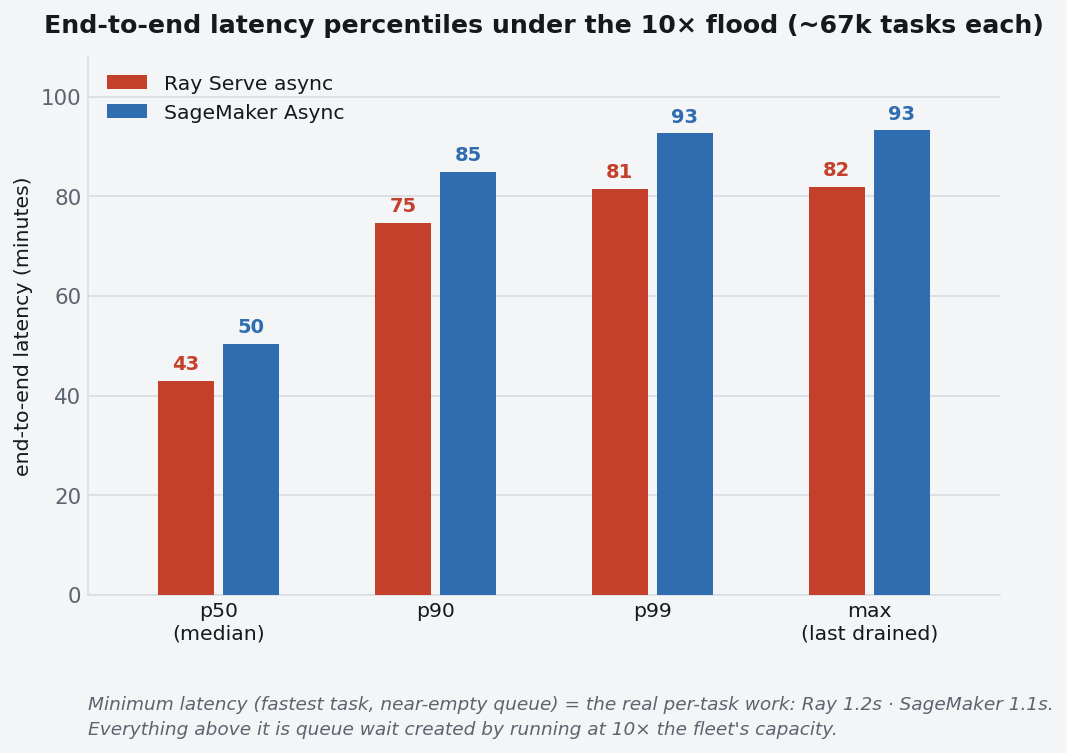
各リクエストには、動画のダウンロード、FFmpeg の実行、埋め込み値の生成、結果の S3 への書き込みを含む約 1〜2 秒の基本処理時間が含まれていました。この部分は両プラットフォームでほぼ同じでした。決定的な違いはキューでの待機時間にあります。利用可能な GPU の数が限られているため、リクエストは処理を開始する前に空き GPU を待つ必要があります。キュー内で待機する時間が長くなるほど、全体のレイテンシは高くなります。
Ray Serve は、蓄積されたバックログに対してより迅速に対応し、SageMaker よりも早く新しいレプリカを起動しました。その結果、リクエストがキューで待たされる時間が短縮され、ユーザーはより早く結果を受け取ることができました。
非同期推論が適しているケース
非同期推論は、処理に時間がかかるワークロードや、HTTP 接続を維持することが現実的ではない場合に有効です。また、急激なトラフィックの増加に対応するワークロードにも適しています。リクエストはキューに待機し、リソースが利用可能になるまで待ちます。
Ray Serve を使えば、わずかな設定で、リクエストのキューイング、信頼性の高い処理、そしてキューサイズに基づく自動スケーリングを実現できます。非同期推論機能は Ray Serve に組み込まれているため、コードを変更することなく、あらゆるクラウド環境やオンプレミス、さらにはノートパソコン上でも同じアプリケーションを動作させることが可能です。
この機能は現在、Ray Serve で利用可能です。詳細については Ray Serve のドキュメント をご覧ください。
リンク参照
- Ray Serve: 自動スケーリング、非同期推論、カスタムルーティング - この記事で構築する機能を紹介した記事。
- Ray Serve: 非同期推論(ドキュメント)
- Amazon SageMaker 非同期推論(概要)
- 非同期エンドポイントの自動スケーリング(Amazon SageMaker)
- SageMaker 推論が生成 AI モデル向けに高速な自動スケーリングを開始
SageMaker サポート機能マトリックス - 非同期推論は単一コンテナのみ対応のため、比較には単一の統合デプロイを使用しています。
原文を表示
*In an *earlier post*, we introduced asynchronous inference in Ray Serve: a way to run long-running model calls off the request path, backed by a message queue, with automatic retries and queue-depth autoscaling. This post is a practical follow-up. We build a real service on top of that feature, a video-indexing pipeline, run it under a heavy load, and compare it against a common managed alternative.*
LinkA quick recap: what async inference is for
In serving ML models, some applications make a single model call that runs for several seconds to minutes, e.g. - transcribing an hour of audio, indexing a video, or generating an image or a video. On a normal synchronous HTTP endpoint the request stays open for the whole computation. At millisecond latencies that coupling is invisible, but for calls this long it creates two problems.
First, a burst of traffic piles onto a fleet that takes seconds or minutes to finish each request, so the workers fall behind and clients, or any intermediary hop, start timing out. Also, a connection held open for minutes has much more exposure to a dropped packet or a failed hop. As a result, the service and overall system gets less reliable at exactly the moments you can't predict.
Async inference solves these problems by decoupling the request scheduling from the actual computation. The client submits a job and gets an id back right away, the work goes onto a message queue, a pool of workers, autoscaled to the queue depth, processes it in the background, and the client polls for the result.
We covered the API and the design in the earlier post, so here we focus on building a service on top of it, and benchmark it under real-world traffic. The pieces Ray Serve provides, in brief:
- @task_consumer / @task_handler - these decorators turn a deployment method into a background worker that pulls from a queue.
- TaskProcessorConfig - configuration that points your code at a message broker you run (e.g. Redis or RabbitMQ are supported) and adds an at-least-once delivery mechanism, retries, and dead-letter routing.
- enqueue_task_sync(...) - function that submits work from the producer side and returns a task id which client can poll for the result.
- AsyncInferenceAutoscalingPolicy - it is the autoscaling policy that scales the worker pool based on queue depth.
LinkThe application: a video-indexing service
Video indexing is a natural fit for async inference. As each request demands a whole video to download, decode, and embed,it can take seconds to minutes of work, and the traffic tends to arrive in bursts such as a batch upload or a nightly backfill. This video indexing service will take an S3 URI and return a task id immediately, and in the background it downloads the video, splits it into frames with ffmpeg, embeds the frames with SigLIP on a GPU, and writes the vectors back to S3, a pipeline that can take tens of minutes per request.
The application, comprises of three deployments, each scaling on its own signal:
- IndexingIngress (CPU) - this deployment accepts POST /index, enqueues the task sent by the user, and returns the task id.
- VideoIndexConsumer (CPU) - the @task_consumer, it consumes tasks from the queue, and downloads and chunks the video with ffmpeg, then calls the encoder. This is the deployment that autoscales on queue depth.
- VideoEncoder (GPU) - a standard deployment holding the SigLIP neural network. The video index consumer deployment calls it through a handle, so frames move between the two over Ray's RPC rather than the network, and it scales on its own GPU load.
The diagram shows the architecture of the service we deployed and tested; purple boxes denotes the deployments, and yellow ones denote the external systems the service talks to.
*Architecture of the service we deployed and tested*
The producer (the deployment which is accepting the user’s request) is a very simple ingress deployment. It enqueues the task and returns an id, so the caller never waits on the work:
@serve.ingress(fastapi_app)
class IndexingIngress:
    def __init__(self, consumer):
        self.adapter = instantiate_adapter_from_config(PROCESSOR_CONFIG)

    @fastapi_app.post("/index")
    async def index(self, req: IndexRequest):
        result = self.adapter.enqueue_task_sync(
            task_name=TASK_INDEX_VIDEO,
            kwargs={"video_uri": req.video_uri, "video_id": req.video_id},
        )
        return {"task_id": result.id, "status": result.status}
The video index consumer is a simple synchronous Python code. It is idempotent on the video id, chunks the video on CPU, calls the GPU encoder through a handle, and stores the result:
@serve.deployment(ray_actor_options={"num_cpus": FFMPEG_THREADS}, ...)
@task_consumer(task_processor_config=PROCESSOR_CONFIG)
class VideoIndexConsumer:
    def __init__(self, encoder):
        self.encoder = encoder               # GPU DeploymentHandle

    @task_handler(name=TASK_INDEX_VIDEO)
    def index_video(self, video_uri, video_id=None):
        if is_done(video_id):                  # idempotent on redelivery
            return {"status": "skipped_already_indexed"}
        chunks = chunk_video(download(video_uri))         # CPU: ffmpeg
        refs = [self.encoder.remote(c.frames) for c in chunks]
        vectors = [r.result()["frame_embeddings"] for r in refs]
        write_video_embeddings(video_id, vectors)         # store to S3
        mark_done(video_id)
        return {"status": "indexed", "num_chunks": len(chunks)}
Note - For the benchmarks below, we fused the VideoIndexConsumer (CPU) and VideoEncoder (GPU) deployments into a single GPU worker, while keeping the same lightweight ingress in front. We did this to make the comparison as fair as possible and to better match the deployment model supported by the alternative, Amazon SageMaker.
SageMaker does not support deploying these two components as separate CPU and GPU services behind a single endpoint. The only alternative would be to expose them as completely separate endpoints; that route would put SageMaker at a further disadvantage: the intermediate tensors would have to travel between the two endpoints over the network, passed by value, whereas Ray Serve passes them by reference through its shared object store. Therefore, all benchmark results presented below were collected using a two-deployment architecture (the ingress and one fused worker), rather than the three-deployment architecture described above.
LinkBehavior under load
Our goal was to stress-test the service and evaluate both its reliability and performance under sustained overload. Ideally, the service should scale with incoming traffic, process requests as quickly as possible, and do so without dropping user requests.
We evaluate reliability by measuring the number of failed requests during the load test, and performance by observing how the system responds to increasing load — particularly its ability to scale up and down in response to traffic while maintaining throughput and stability.
To exercise both aspects, we ran a 20-minute flood test at a sustained 50 RPS with periodic spikes to 100 RPS. This workload is approximately 5–10× higher than what a 4-GPU fleet can process, resulting in roughly 67,000 video requests over the duration of the test. Since the incoming request rate significantly exceeds the fleet's processing capacity, a request backlog is inevitable, making this a good test of the system's scaling behavior and resilience under sustained pressure.
As a result, we observed
- Replicas scaled with demand - As the backlog grew, the application automatically increased the number of GPU replicas from 1 to 4, which was the configured maximum. Once the backlog was cleared, it scaled back down to 1. There was no fixed fleet and no manual tuning per burst.
- Zero failed requests - All ~67,000 video requests were successfully accepted, queued, and eventually processed. The dead-letter queue remained empty throughout the test, indicating that no requests were dropped or failed during the sustained overload.
LinkComparing against a managed alternative: Amazon SageMaker
To put these numbers in context, we ran the same workload on Amazon SageMaker Async Inference, a common managed solution for this type of workload. Like our setup, SageMaker queues incoming requests, scales based on the backlog, and reads from and writes to S3. Both setups used the same hardware (4× NVIDIA T4 GPUs), the same 1-frame SigLIP workload, and the same 20-minute flood test, with both starting from a single cold instance. Since a SageMaker async endpoint runs a single model container, we used the same single, fused deployment on the Ray Serve side, as described above.
This means the deployment architecture, hardware, and workload were the same on both sides, making the orchestration engine the primary difference between the two systems.
| Metric (same flood, 4x T4) | Ray Serve async | SageMaker Async |
|---|---|---|
| Time to full fleet (cold) | ~155 s | ~589 s |
| Release idle capacity (fastest measured) | ~5 s | ~104 s |
| Autoscaling configuration | 1 policy block | 2 step policies + 2 alarms (explained below)* |
| Failed / lost tasks | 0 | 0 |
| Ack latency, p50 (under load) | 12.8 ms | 11.8 ms |
- We autoscaled the SageMaker endpoint with two Application Auto Scaling step policies, each tied to a CloudWatch alarm. A backlog-fast alarm fires when ApproximateBacklogSizePerInstance hits 5 or more (on a single 60-second datapoint), triggering the fast-out policy to jump straight to the 4-instance cap, and backlog-empty alarm fires when the total ApproximateBacklogSize drops below 1, triggering the fast-in policy to drop back to a single instance.
1 - Offered RPS Graph w.r.t. time.
*Offered load over the 20-minute flood (identical profile for both engines)*
1 - Number of GPU replicas/instances w.r.t. time.
2 - Showing backlog queue length in Ray Serve vs Amazon SageMaker w.r.t time
*Fleet size over the flood, both scale up to 4 and release back to 1*
Below are the few observations from the above runs:
- Scale-up is close. Both reach a full 4-GPU fleet in the same ballpark, and most of that time went to node provisioning, which both pay. The difference is in the decision to scale: Ray Serve polls the queue depth directly and reacts in seconds, while SageMaker's decision is bounded by the resolution of its CloudWatch metric.
- Scale-down differs more. Once the queue was empty, Ray Serve scaled back down within a few seconds. The fastest scale-down we saw with SageMaker was about 104 seconds.
- Ray Serve was easier to set up. The Ray Serve side is one autoscaling policy block. To get similar behavior in SageMaker, we had to configure multiple autoscaling policies and several CloudWatch alarms.
- Neither dropped anything. Both processed the full flood with an empty dead-letter queue.
A note on the SageMaker setup: autoscaling is configured to be as responsive as the platform allows. It uses a single 60-second CloudWatch alarm on the ApproximateBacklogSize and ApproximateBacklogSizePerInstance metric to trigger both scale-out and scale-in actions. Faster scaling isn't possible because these metrics are standard-resolution metric, so CloudWatch alarms cannot evaluate it more frequently than once every 60 seconds.
LinkEnd-to-end latency
Scaling speed is only part of the story. Another is - how long a user has to wait for their request to finish end to end. To measure this, we tracked the time from when a video was submitted until its embeddings were written to S3 for every request in the flood test, and below are the results:.
Each request had a base processing time of about 1–2 seconds, which included downloading the video, running FFmpeg, generating embeddings, and writing the results to S3. This part was nearly the same on both platforms. The difference came from waiting in the queue. Since there were only a limited number of GPUs available, requests had to wait for a free GPU before they could be processed. The longer a request waits in the queue, the higher its overall latency.
Ray Serve responded to the growing backlog more quickly and started new replicas sooner than SageMaker. As a result, requests spent less time waiting in the queue, so users received their results earlier.
LinkWhen async inference is the right fit
Async inference is useful for workloads that take longer to finish and where keeping an HTTP connection open is not practical. It is also a good fit for workloads with sudden traffic spikes, since requests can wait in a queue until resources are available. With Ray Serve, you get request queuing, reliable request processing, and automatic scaling based on queue size with just a small amount of configuration. Since it is built into Ray Serve, the same application can run on any cloud, on-premises, or even on a laptop without code changes.
The feature is available in Ray Serve today; You can find more details in the Ray Serve documentation.
LinkReferences
- Ray Serve: autoscaling, async inference, and custom routing - the post that introduced the feature this one builds on.
- Ray Serve: Asynchronous Inference (documentation)
- Amazon SageMaker Asynchronous Inference (overview)
- Autoscale an asynchronous endpoint (Amazon SageMaker)
- SageMaker inference launches faster auto scaling for generative AI models
SageMaker supported-features matrix - async inference is single-container, which is why the comparison used a single collapsed deployment.
今日のまとめ
AIデイリーブリーフで今日の重要ニュースをまとめ読み