なぜ私のモデルは機能しないのか？

imageHave you ever trained a model you thought was good, but then it failed miserably when applied to real world data? If so, you’re in good company. Machine learning processes are complex, and it’s very easy to do things that will cause overfitting without it being obvious. In the 20 years or so that I’ve been working in machine learning, I’ve seen many examples of this, prompting me to write “How to avoid machine learning pitfalls: a guide for academic researchers” in an attempt to prevent other people from falling into these traps.

But you don’t have to take my word for it. These issues are being increasingly reported in both the scientific and popular press. Examples include the observation that hundreds of models developed during the Covid pandemic simply don’t work, and that a water quality system deployed in Toronto regularly told people it was safe to bathe in dangerous water. Many of these are documented in the AIAAIC repository. It’s even been suggested that these machine learning missteps are causing a reproducibility crisis in science — and, given that many scientists use machine learning as a key tool these days, a lack of trust in published scientific results.

In this article, I’m going to talk about some of the issues that can cause a model to seem good when it isn’t. I’ll also talk about some of the ways in which these kinds of mistakes can be prevented, including the use of the recently-introduced REFORMS checklist for doing ML-based science.

Duped by Data

Misleading data is a good place to start, or rather not a good place to start, since the whole machine learning process rests upon the data that’s used to train and test the model.

In the worst cases, misleading data can cause the phenomenon known as garbage in garbage out; that is, you can train a model, and potentially get very good performance on the test set, but the model has no real world utility. Examples of this can be found in the aforementioned review of Covid prediction models by Roberts et al. In the rush to develop tools for Covid prediction, a number of public datasets became available, but these were later found to contain misleading signals — such as overlapping records, mislabellings and hidden variables — all of which helped models to accurately predict the class labels without learning anything useful in the process.

Take hidden variables. These are features that are present in data, and which happen to be predictive of class labels within the data, but which are not directly related to them. If your model latches on to these during training, it will appear to work well, but may not work on new data. For example, in many Covid chest imaging datasets, the orientation of the body is a hidden variable: people who were sick were more likely to have been scanned lying down, whereas those who were standing tended to be healthy. Because they learnt this hidden variable, rather than the true features of the disease, many Covid machine learning models turned out to be good at predicting posture, but bad at predicting Covid. Despite their name, these hidden variables are often in plain sight, and there have been many examples of classifiers latching onto boundary markers, watermarks and timestamps embedded in images, which often serve to distinguish one class from another without having to look at the actual data.

A related issue is the presence of spurious correlations. Unlike hidden variables, these have no true relationship to anything else in the data; they’re just patterns that happen to correlate with the class labels. A classic example is the tank problem, where the US military allegedly tried to train a neural network to identify tanks, but it actually recognised the weather, since all the pictures of tanks were taken at the same time of day. Consider the images below: a machine learning model could recognise all the pictures of tanks in this dataset just by looking at the colour of pixels towards the top of an image, without having to consider the shape of any of the objects. The performance of the model would appear great, but it would be completely useless in practice.

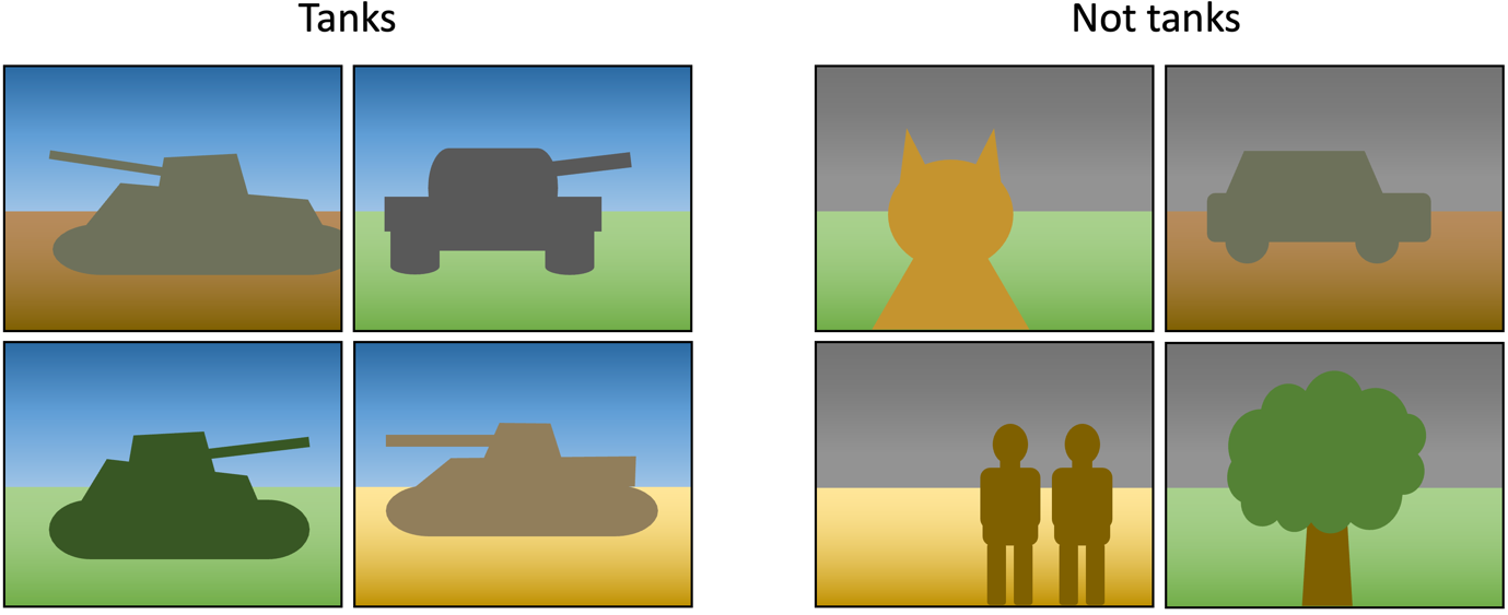image(Source: by author)Many (perhaps most) datasets contain spurious correlations, but they’re not usually as obvious as this one. Common computer vision benchmarks, for example, are known to have groups of background pixels that are spuriously correlated with class labels. This represents a particular challenge to deep learners, which have the capacity to model many patterns within the data; various studies have shown that they do tend to capture spuriously correlated patterns, and this reduces their generality. Sensitivity to adversarial attacks is one consequence of this: if a deep learning model bases its prediction on spurious correlations in the background pixels of an image, then making small changes to these pixels can flip the prediction of the model. Adversarial training, where a model is exposed to adversarial samples during training, can be used to address this, but it’s expensive. An easier approach is just to look at your model, and see what information it’s using to make its decisions. For instance, if a saliency map produced by an explainable AI technique suggests that your model is focusing on something in the background, then it’s probably not going to generalise well.

Sometimes it’s not the data itself that is problematic, but rather the labelling of the data. This is especially the case when data is labelled by humans, and the labels end up capturing biases, misassumptions or just plain old mistakes made by the labellers. Examples of this can be seen in datasets used as image classification benchmarks, such as MNIST and CIFAR, which typically have a mislabelling rate of a couple of percent — not a huge amount, but pretty significant where modellers are fighting over accuracies in the tenths of a percent. That is, if your model does slightly better than the competition, is it due to an actual improvement, or due to modelling noise in the labelling process? Things can be even more troublesome when working with data that has implicit subjectivity, such as sentiment classification, where there’s a danger of overfitting particular labellers.

Led by Leaks

Bad data isn’t the only problem. There’s plenty of scope for mistakes further down the machine learning pipeline. A common one is data leakage. This happens when the model training pipeline has access to information it shouldn’t have access to, particularly information that confers an advantage to the model. Most of the time, this manifests as information leaks from the test data — and whilst most people know that test data should be kept independent and not explicitly used during training, there are various subtle ways that information can leak out.

One example is performing a data-dependent preprocessing operation on an entire dataset, before splitting off the test data. That is, making changes to all the data using information that was learnt by looking at all the data. Such operations vary from the simple, such as centering and scaling numerical features, to the complex, such as feature selection, dimensionality reduction and data augmentation — but they all have in common the fact that they use knowledge of the whole dataset to guide their outcome. This means that knowledge of the test data is implicitly entering the model training pipeline, even if it is not explicitly used to train the model. As a consequence, any measure of performance derived from the test set is likely to be an overestimate of the model’s true performance.

Let’s consider the simplest example: centering and scaling. This involves looking at the range of each feature, and then using this information to rescale all the values, typically so that the mean is 0 and the standard deviation is 1. If this is done on the whole dataset before splitting off the test data, then the scaling of the training data will include information about the range and distribution of the feature values in the test set. This is particularly problematic if the range of the test set is broader than the training set, since the model could potentially infer this fact from the truncated range of values present in the training data, and do well on the test set just by predicting values higher or lower than those which were seen during training. For instance, if you’re working on stock price forecasting from time series data with a model that takes inputs in the range 0 to 1 but it only sees values in the range 0 to 0.5 during training, then it’s not too hard for it to infer that stock prices will go up in the future.

In fact, forecasting is an area of machine learning that is particularly susceptible to data leaks, due to something called look ahead bias. This occurs when information the model shouldn’t have access to leaks from the future and artificially improves its performance on the test set. This commonly happens when the training set contains samples that are further ahead in time than the test set. I’ll give an example later of when this can happen, but if you work in this area, I’d also strongly recommend taking a look at this excellent review of pitfalls and best practices in evaluating time series forecasting models.

An example of a more complex data-dependent preprocessing operation leading to overly-optimistic performance metrics can be found in this review of pre-term birth prediction models. Basically, a host of papers reported high accuracies at predicting whether a baby would be born early, but it turned out that all had applied data augmentation to the data set before splitting off the test data. This resulted in the test set containing augmented samples of training data, and the training set containing augmented samples of test data — which amounted to a pretty significant data leak. When the authors of the review corrected this, the predictive performance of the models dropped from being near perfect to not much better than random.

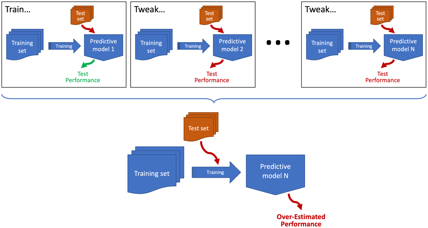image(Source: https://arxiv.org/abs/2108.02497)Oddly, one of the most common examples of data leakage doesn’t have an agreed name (the terms overhyping and sequential overfitting have been suggested) but is essentially a form of training to the test set. By way of example, imagine the scenario depicted above where you’ve trained a model and evaluated it on the test set. You then decided its performance was below where you wanted it to be. So, you tweaked the model, and then you reevaluated it. You still weren’t happy, so you kept on doing this until its performance on the test set was good enough. Sounds familiar? Well, this is a common thing to do, but if you’re developing a model iteratively and using the same test set to evaluate the model after each iteration, then you’re basically using that test set to guide the development of the model. The end result is that you’ll overfit the test set and probably get an over-optimistic measure of how well your model generalises.

Interestingly, the same process occurs when people use community benchmarks, such as MNIST, CIFAR and ImageNet. Almost everyone who works on image classification uses these data sets to benchmark their approaches; so, over time, it’s inevitable that some overfitting of these benchmarks will occur. To mitigate against this, it’s always advisable to use a diverse selection of benchmarks, and ideally try your technique on a data set which other people haven’t used.

Misinformed by Metrics

Once you’ve built your model robustly, you then have to evaluate it robustly. There’s plenty that can go wrong here too. Let’s start with an inappropriate choice of metrics. The classic example is using accuracy with an imbalanced dataset. Imagine that you’ve managed to train a model that always predicts the same label, regardless of its input. If half of the test samples have this label as their ground truth, then you’ll get an accuracy of 50% — which is fine, a bad accuracy for a bad classifier. If 90% of the test samples have this label, then you’ll get an accuracy of 90% — a good accuracy for a bad classifier. This level of imbalance is not uncommon in real world data sets, and when working with imbalanced training sets, it’s not uncommon to get classifiers that always predict the majority label. In this case, it would be much better to use a metric like F score or Matthews correlation coefficient, since these are less sensitive to class imbalances. However, all metrics have their weaknesses, so it’s always best to use a portfolio of metrics that give different perspectives on a model’s performance and failure modes.

Metrics for time series forecasting are particularly troublesome. There are a lot of them to choose from, and the most appropriate choice can depend on both the specific problem domain and the exact nature of the time series data. Unlike metrics used for classification, many of the regression metrics used in time series forecasting have no natural scale, meaning that raw numbers can be misleading. For instance, the interpretation of mean squared errors depends on the range of values present in the time series. For this reason, it’s important to use appropriate baselines in addition to appropriate metrics. As an example, this (already mentioned) review of time series forecasting pitfalls demonstrates how many of the deep learning models published at top AI venues are actually less good than naive baseline models. For instance, they show that an autoformer, a kind of complex transformer model designed for time series forecasting, can be beaten by a trivial model that predicts no change at the next time step — something that isn’t apparent from looking at metrics alone.

In general, there is a trend towards developing increasingly complex models to solve difficult problems. However, it’s important to bear in mind that some problems may not be solvable, regardless of how complex the model becomes. This is probably the case for many financial time series forecasting problems. It’s also the case when predicting certain natural phenomena, particularly those in which a chaotic component precludes prediction beyond a certain time horizon. For instance, many people think that earthquakes can not be predicted, yet there are a host of papers reporting good performance on this task. This review paper discusses how these correct predictions may be due to a raft of modelling pitfalls, including inappropriate choice of baselines and overfitting due to data sparsity, unnecessary complexity and data leaks.

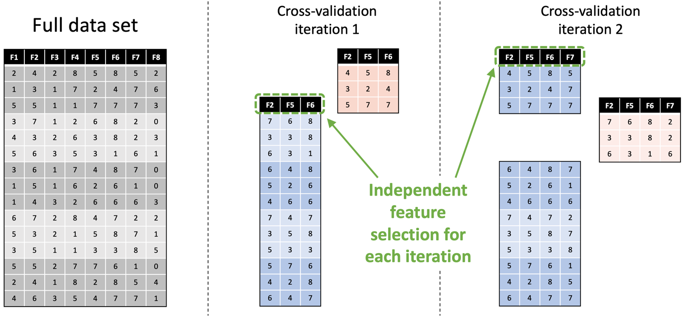
Another problem is assuming that a single evaluation is sufficient to measure the performance of a model. Sometimes it is, but a lot of the time you’ll be working with models that are stochastic or unstable; so, each time you train them, you get different results. Or you may be working with a small data set where you might just get lucky with an easy test split. To address both situations, it is commonplace to use resampling methods like cross-validation, which train and test a model on different subsets of the data and then work out the average performance. However, resampling introduces its own risks. One of these is the increased risk of data leaks, particularly when assuming that data-dependent preprocessing operations (like centering and scaling and feature selection) only need to be done once. They don’t; they need to be done independently for each iteration of the resampling process, and to do otherwise can cause a data leak. Below is an example of this, showing how feature selection should be done independently on the two training sets (in blue) used in the first two iterations of cross-validation, and how this results in different features being selected each time.

image(Source: https://arxiv.org/abs/2108.02497)As I mentioned earlier, the danger of data leaks is even greater when working with time series data. Using standard cross-validation, every iteration except one will involve using at least one training fold that is further ahead in time than the data in the test fold. For example, if you imagine that the data rows in the figure above represent time-ordered multivariate samples, then the test sets (in pink) used in both iterations occur earlier in the time series than all or part of the training data. This is an example of a look ahead bias. Alternative approaches, such as blocked cross-validation, can be used to prevent these.

Multiple evaluations aren’t an option for everyone. For example, training a foundation model is both time-consuming and expensive, so doing it repeatedly is not feasible. Depending on your resources, this may be the case for even relatively small deep learning models. If so, then also consider using other methods for measuring the robustness of models. This includes things like using explainability analysis, performing ablation studies, or augmenting test data. These can allow you to look beyond potentially-misleading metrics and gain some appreciation of how a model works and how it might fail, which in turn can help you decide whether to use it in practice.

Falling Deeper

So far, I’ve mostly talked about general machine learning processes, but the pitfalls can be even greater when using deep learning models. Consider the use of latent space models. These are often trained separately to the predictive models that use them. That is, it’s not unusual to train something like an autoencoder to do feature extraction, and then use the output of this model within the training of a downstream model. When doing this, it’s essential to ensure that the test set used in the downstream model does not intersect with the training data used in the autoencoder — something that can easily happen when using cross-validation or other resampling methods, e.g. when using different random splits or not selecting models trained on the same training folds.

However, as deep learning models get larger and more complex, it can be harder to ensure these kinds of data leaks do not occur. For instance, if you use a pre-trained foundation model, it may not be possible to tell whether the data used in your test set was used to train the foundation model — particularly if you’re using benchmark data from the internet to test your model. Things get even worse if you’re using composite models. For example, if you’re using a BERT-type foundation model to encode the inputs when fine-tuning a GPT-type foundation model, you have to take into account any intersection between the datasets used to train the two foundation models in addition to your own fine-tuning data. In practice, some of these data sets may be unknown, meaning that you can’t be confident whether your model is correctly generalising or merely reproducing data memorised during pre-training.

Avoiding the Pits

These pitfalls are all too common. So, what’s the best way to avoid them? Well, one thing you can do is use a checklist, which is basically a formal document that takes you through the key pain points in the machine learning pipeline, and helps you to identify potential issues. In domains with high-stakes decisions, such as medicine, there are already a number of well-established checklists, such as CLAIM, and adherence to these is typically enforced by journals that publish in these areas.

However, I’d like to briefly introduce a new kid on the block: REFORMS, a consensus-based checklist for doing machine learning-based science. This was put together by 19 researchers across computer science, data science, mathematics, social sciences, and the biomedical sciences — including myself — and came out of a recent workshop on the reproducibility crisis in ML‑based science. It is intended to address the common mistakes