METR、エージェント能力を評価する指標「Metrics of Agent Ability」を発表

.post-content .metrics-agent-note { --metrics-font: system-ui, -apple-system, "Segoe UI", Roboto, "Helvetica Neue", "Noto Sans", "Liberation Sans", Arial, sans-serif, "Apple Color Emoji", "Segoe UI Emoji", "Segoe UI Symbol", "Noto Color Emoji"; --metrics-column-gap: min(4vw, 1.5em); color: #212529; font-family: var(--metrics-font); font-size: 14.6667px; line-height: 1.5; } .post-content .metrics-agent-note :where(p, li, dt, dd, table, th, td, label) { font-family: var(--metrics-font); } .post-content .metrics-agent-note p, .post-content .metrics-agent-note li { font-size: 13.2px; line-height: 1.5; } .post-content .metrics-agent-note p { margin: 0 0 14.6667px; padding-top: 7.3333px; } .post-content .metrics-agent-note li { margin: 0; } .post-content .metrics-agent-note ul, .post-content .metrics-agent-note ol { margin: 0 0 14.6667px 1.5rem; padding-left: 1rem; } .post-content .metrics-agent-note ul ul, .post-content .metrics-agent-note ol ol, .post-content .metrics-agent-note ul ol, .post-content .metrics-agent-note ol ul { margin-bottom: 0; } .post-content .metrics-agent-note h1, .post-content .metrics-agent-note h2, .post-content .metrics-agent-note h3, .post-content .metrics-agent-note h4 { color: #212529; font-family: var(--metrics-font); font-weight: 600; text-wrap: wrap; } .post-content .metrics-agent-note h1 { border-bottom: 8px solid #557; font-size: 23.3753px; line-height: 1.2; margin: 29.3333px 0 14.6667px; padding: 0; } .post-content .metrics-agent-note h2 { border-bottom: 1px solid #ccc; font-size: 21.0224px; line-height: 1.2; margin: 14.6667px 0; padding: 0 0 7.3333px; } .post-content .metrics-agent-note h3 { font-size: 17px; margin: 14.6667px 0 7.3333px; } .post-content .metrics-agent-note a { text-decoration: underline; } .post-content .metrics-agent-note .canonical-note { color: #555; margin-bottom: 1.25rem; } .post-content .metrics-agent-note .metric-row { align-items: flex-start; display: flex; gap: var(--metrics-column-gap); } .post-content .metrics-agent-note .metric-figure-column { flex: 2 1 0; min-width: 0; } .post-content .metrics-agent-note .metric-copy-column { flex: 3 1 0; min-width: 0; } .post-content .metrics-agent-note .metric-figure-column > p { margin: 0; padding: 0; } .post-content .metrics-agent-note figure { margin: 14.6667px 0; text-align: center; } .post-content .metrics-agent-note figure img { display: block; height: auto; margin: 0 auto; max-width: 100%; } .post-content .metrics-agent-note figure figcaption { color: #555; font-family: var(--metrics-font); font-size: 12px; line-height: 1.4; margin-top: 7.3333px; text-align: center; } .post-content .metrics-agent-note dl { display: block; margin: 0 0 14.6667px; } .post-content .metrics-agent-note dt { font-weight: 600; } .post-content .metrics-agent-note #faq-notes ~ dl dt { font-weight: 600; } .post-content .metrics-agent-note dd { font-size: 13.2px; line-height: 1.5; margin: 0 0 7.3333px 2em; } .post-content .metrics-agent-note table { border-collapse: collapse; display: block; font-size: 14.6667px; line-height: 1.5; margin: 7.3333px 0; max-width: 100%; overflow-x: auto; width: 100%; } .post-content .metrics-agent-note .objects-intro { margin-bottom: 0; } .post-content .metrics-agent-note table.objects-table { margin-top: 0; } .post-content .metrics-agent-note table.objects-table thead { display: none; } .post-content .metrics-agent-note th, .post-content .metrics-agent-note td { border-left: 0 !important; border-right: 0 !important; border-top: 0 !important; border-bottom: 1px solid #dee2e6; padding: 7.3333px; text-align: left; vertical-align: top; } .post-content .metrics-agent-note thead th { border-bottom-width: 2px; } .post-content .metrics-agent-note .math.display { display: block; overflow-x: auto; padding: 0.25rem 0; } .post-content .metrics-agent-note .references .csl-entry { clear: both; font-size: 13.2px; margin-bottom: 0.5em; } .post-content .metrics-agent-note .hanging-indent .csl-entry { margin-left: 2em; text-indent: -2em; } .post-content .metrics-agent-note .footnotes { border-top: 1px solid #dee2e6; margin-top: 2rem; padding-top: 0.5rem; } .post-content .metrics-agent-note .footnotes ol { margin-left: 1rem; } @media (min-width: 768px) { .post-content .metrics-agent-note dl { align-items: baseline; column-gap: var(--metrics-column-gap); display: grid; grid-template-columns: minmax(0, 2fr) minmax(0, 3fr); row-gap: 0.5em; } .post-content .metrics-agent-note dt { grid-column: 1; } .post-content .metrics-agent-note dd { grid-column: 2; margin-left: 0; } } @media (max-width: 767px) { .post-content .metrics-agent-note .metric-row { display: block; } .post-content .metrics-agent-note .metric-figure-column, .post-content .metrics-agent-note .metric-copy-column { width: 100%; } .post-content .metrics-agent-note .metric-figure-column { margin-bottom: 0.75rem; } .post-content .metrics-agent-note h1 { font-size: 21px; } .post-content .metrics-agent-note h2 { font-size: 19px; } } .post-content .metrics-agent-note img.metric-figure { display: block; height: auto; margin: 0 auto; max-width: 100%; width: 100%; } .post-content .metrics-agent-note blockquote.metrics-callout { background: #f8fbff; border: 1px solid #9ec5fe; border-left: 5px solid #0d6efd; border-radius: 0.25rem; margin: 18.3333px 0; padding: 0 0.75rem 0.5rem; } .post-content .metrics-agent-note blockquote.metrics-callout::before, .post-content .metrics-agent-note blockquote.metrics-callout::after { content: none; } .post-content .metrics-agent-note blockquote.metrics-callout > p:first-child { background: #cfe2ff; font-size: 14.6667px; margin: 0 -0.75rem 0.25rem; padding: 0.5rem 0.75rem; } .post-content .metrics-agent-note .csl-entry { font-size: 13.2px; margin-bottom: 0.5em; margin-left: 2em; text-indent: -2em; } Goals of this post > > Goal: a simple way to compare a variety of capability metrics in an idealized setting where we observe only a function from $x$ to $s$. > > Non-goals: > > 1. Treatment of practical difficulties (an incomplete list of other considerations appears at the bottom). > 2. Recommendations about which metric to use. > 3. Representation of a consensus METR view. {: .metrics-callout} --> This post reviews alternative metrics of agent capability. This post contains a fairly comprehensive taxonomy of capability metrics for the situation in which you observe score curves for an agent and a human. Every metric is based off the following two score functions:

$s_A(x)$ = agent score as a function of expenditure

$s_H(x)$ = human score as a function of expenditure

Expenditure can be interpreted as money spent, or tokens, or time required.

What I will not do. I will generally not give recommendations of which metric is the best for which situation. I will not give a deep discussion of how to measure the score curves, $s_H$ and $s_A$. There are many practical difficulties involved in this.

I will generally address only scores on a single task; applications to collections of tasks (benchmark scores) can be a bit more complicated.

I will mostly not discuss other desirable properties of metrics - e.g. whether it is understandable, whether it is generalizable.

Some general observations. Some personal observations that I think are fairly natural: If score curves are very concave (meaning score is invariant to expenditure) then just reporting the raw score is fine, given some reasonable amount of expenditure.

If score curves show high returns to expenditure then we need a metric that takes into account test-time scaling.

Benchmarking against human abilities helps us generalize to entirely new tasks.

As the models get very good then many of the human-relevant benchmarks become no longer useful.

Setup and Definitions

image

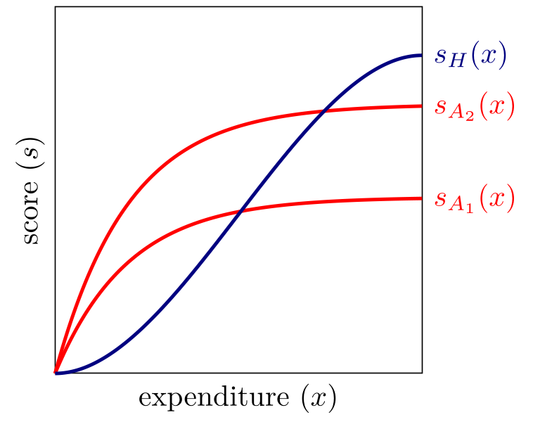
Each agent and each human is characterized by a function from expenditure to score, $s(x)$, and $s^{-1}(\bar{s})$ represents the expenditure required to reach a score $\bar{s}$.

In general I interpret score as performance on a single task, e.g., the speedup on an optimization problem. We could also interpret score as the share of binary tasks completed, or the probability of completing a single task.1

Expenditure will generally be treated as money, but it can also be interpreted as time or tokens.

Human-grounded metrics that compare agent and human expenditure require both expenditures to be measured in the same units or converted into a common unit such as dollars.

I will typically draw the agent curves ($s_A(\cdot)$) as more concave than the human curves ($s_H(\cdot)$).2 I think this accurately represents the reality for most tasks today (e.g., Wijk et al. (2025)), but it could change.

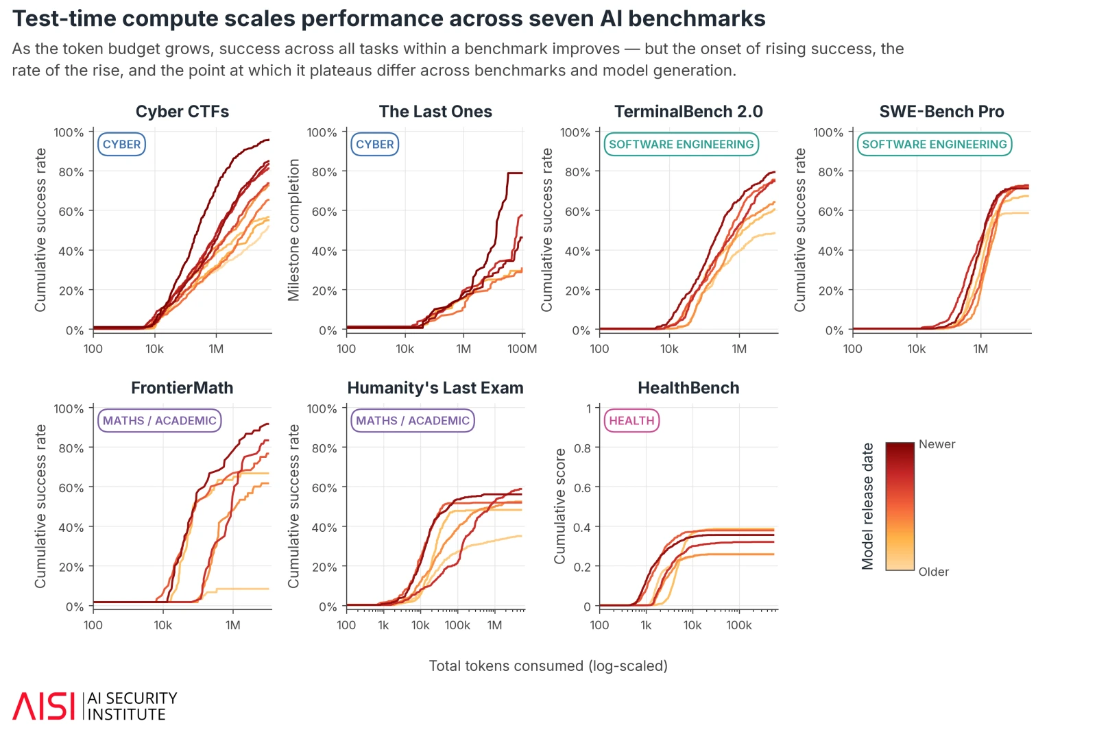
AISI’s recent post on More test-time compute, more capability has a good discussion and visualization of test-time scaling curves across a variety of different benchmarks:

image

Agent-Only Metrics of Ability

We first discuss metrics that depend only on the agent’s score, without benchmarking against humans.3

Score at Fixed Expenditure

image

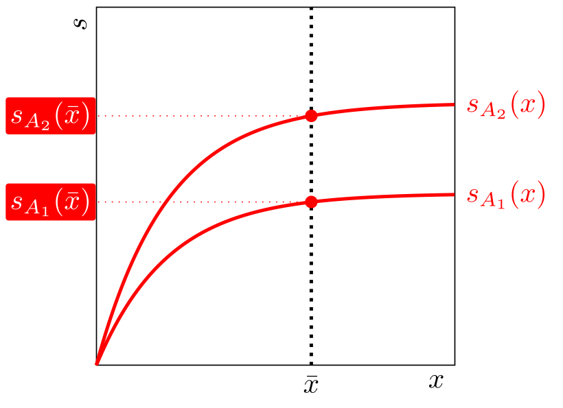
This is the typical way we report most evals: pick a fixed expenditure $\bar{x}$ and report each agent’s score $s_A(\bar{x})$. If $s_A(\cdot)$ reliably asymptotes at a fairly low value of $x$, then this is a sufficient statistic for most purposes.

This metric becomes less useful when agent scores continue increasing even at high levels of expenditure; e.g., see the criticisms by Noam Brown and Kapoor et al. (2025).4

Another reason for fixing expenditure is to increase separation in scores, where a higher level of expenditure would cause saturation, and so little discrimination between model capabilities (e.g. in a recent AISI post).5

Score at Practical Plateau

image

A common practical response is to report the score at the point where the function plateaus, or falls below a certain slope (assuming concavity). E.g., Kwa and West et al. (2025) say “Models were given sufficiently high token limits to reach a plateau in success rate.”

This is roughly equivalent to reporting score at a high expenditure level, representing the highest reasonable level of expenditure. It will not be well-defined if the score function never plateaus.

Expenditure at Fixed Score

image

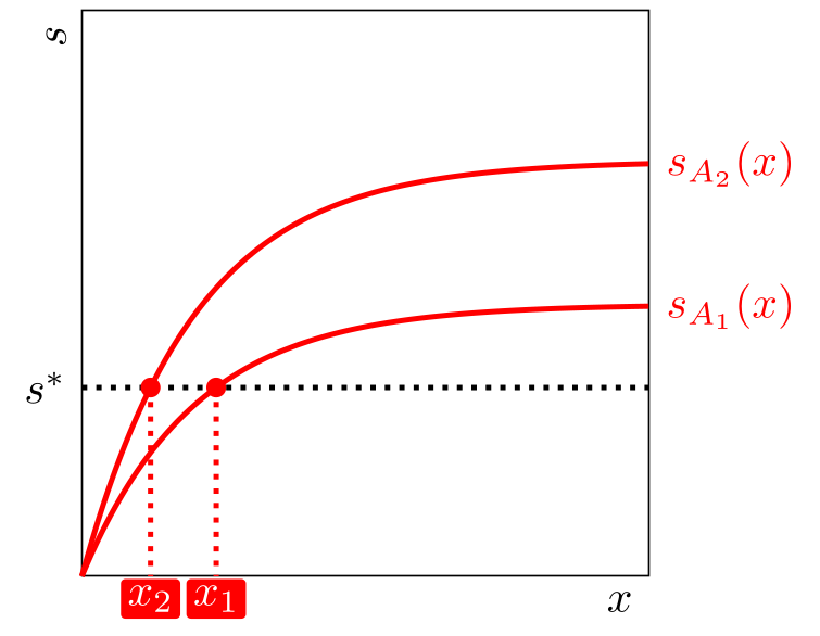
We can instead fix a target score $\bar{s}$ and report the infimum expenditure needed to reach that score: $x=s_{A}^{-1}(\bar{s})$.

This metric will only give a finite number if the evaluated model can achieve the score $\bar{s}$. This is a cost-efficiency metric, often used when looking at declines in model costs over time (Gundlach et al. 2026; Cottier et al. 2025).6

If agents all had the same relative costs of performance, then new generations of models would shift multiplicatively left (additively left in log-space), and this type of “efficiency” metric would be a sufficient statistic for ability. However, there is some reason to believe that new models typically have disproportionate impacts at high expenditures, i.e. they make certain scores available that would have been almost impossible at any expenditure for an earlier model.7

Returns to Expenditure

image

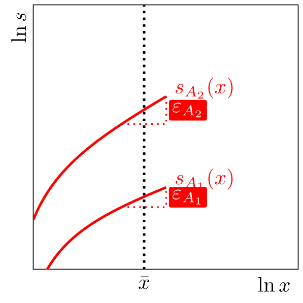
If the returns to expenditure do not plateau, even at significant levels of expenditure, then score at a fixed expenditure is not a satisfactory metric.

Instead, it can be useful for a metric to express the marginal returns to expenditure. The nature of the scaling can vary across domains, and so the appropriate metric is often chosen depending on the shape of the scaling. Two common patterns:

Log-linear scaling: Many test-time scaling results claim roughly log-linear scaling.8

Log-log scaling: If the returns to expenditure are a power law, then the elasticity (ratio of log changes) will be constant. This is a common metric for expressing the returns to human effort, e.g., in the R&D production function of Jones (1995).

In each case the relationship will be linear on a graph with appropriately transformed axes. However it’s also possible that no consistent relationship exists.

Expenditure-Adjusted Score

image

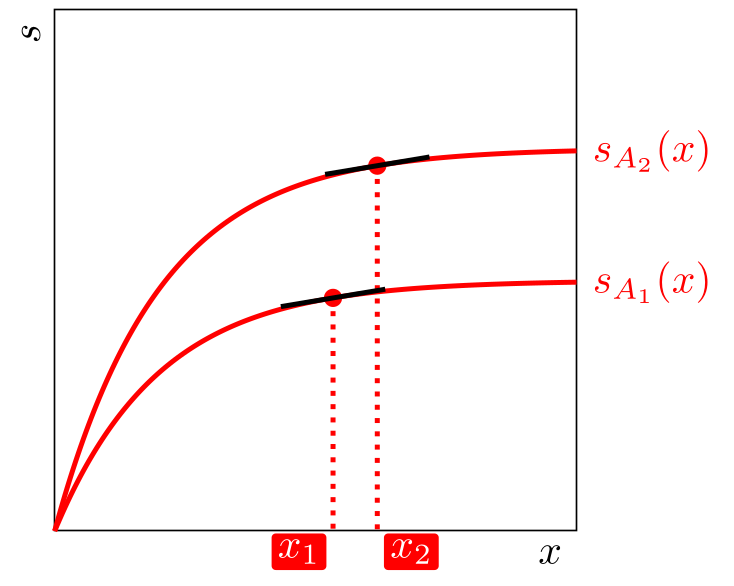
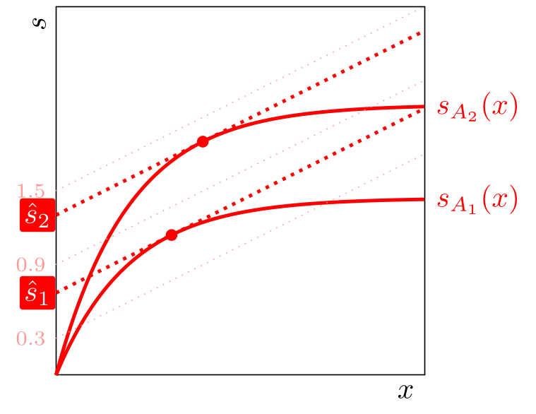
If we are willing to be opinionated about the relative value of expenditure and score, then we can express those tradeoffs with a utility function $U(s,x)$, which will give us a metric of value. Each agent will have a different level of optimal expenditure (represented by a tangency point on the diagram) and a different level of utility.

The utility can be expressed as an expenditure-adjusted score: the score at zero expenditure that would make you indifferent between receiving that score and using the agent at its optimal expenditure:

\[\hat{s}_A:\quad U(\hat{s}_A,0)=\max_{x\geq 0} U(s_A(x),x).\] The utility can also be expressed in monetary units, representing the total value you get from using the agent. Visually this will be the intersection of the optimal indifference curve with the $x$-axis (not pictured, it would fall on the negative part of the $x$-axis).

\[\hat{x}_A:\quad U(0,-\hat{x}_A)=\max_{x\geq 0} U(s_A(x),x).\]

Human-Grounded Metrics

Calibrating against human effort. We now discuss a set of metrics which are calibrated against human effort. An advantage of human-grounded metrics is their interpretability and generalizability. If an agent’s human-equivalent time horizon were stable across tasks, it would allow us to predict its performance on a new task without first testing the agent on that task. A natural metric for human expenditure is time spent on the problem, and so some of these metrics use human-equivalent time as a metric of agent capability. However, if we are comparing agent and human expenditure on the same axes, then money is a more natural interpretation of $x$.

Binary Time Horizon

image

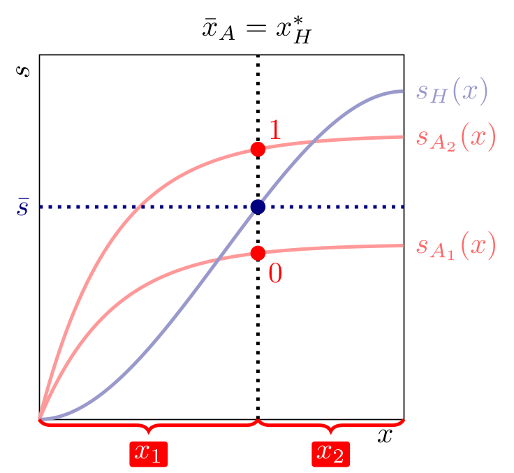
Many continuously-scored tasks grade agents by a single human expenditure threshold. E.g. the Opus 5 system card reports a series of AI R&D tasks, and for each a score that was achieved by a human after a specific amount of time (e.g. 8 hours or 40 hours). Agents can then be graded as passing if they beat the baseline.

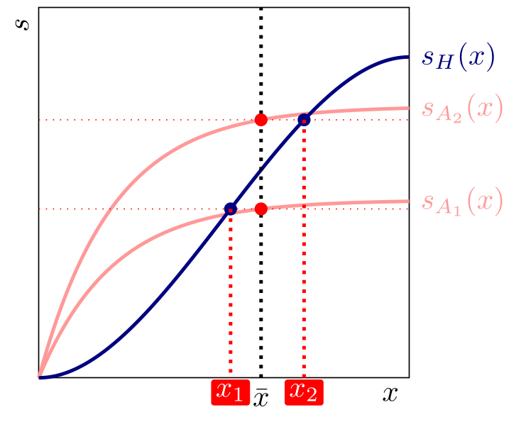
METR’s “time horizon” metric (Kwa and West et al. (2025)) combines many binary scores into a human-equivalent time for each model, based on the $x$ at which the agent matches or exceeds the human score half the time.9

Formally, for each task we choose a reference score \(\bar{s}\) and calculate the infimum human expenditure \(x_H^*=s_H^{-1}(\bar{s})\) needed to achieve that score. Here expenditure is measured in time, but it could also be measured in money.

We then calculate the agent’s score at some fixed expenditure \(\bar{x}_A\), and give the agent a binary score based on whether \(s_A(\bar{x}_A)\) is above or below \(\bar{s}\).

The diagram shows equal expenditure on humans and agents (\(\bar{x}_A=x_H^*\)). The fixed agent expenditure \(\bar{x}_A\) need not equal the human expenditure \(x_H^*\), but equal expenditure on each is a natural choice for interpretability.

Continuous Time Horizon

image

We can extend the time horizon metric by retaining the agent’s continuous score rather than reducing it to a binary comparison.

We elicit each agent at a single expenditure level, $\bar{x}_A$, and then compare the resulting score with the whole human curve, rather than with one binary threshold.

The human-equivalent expenditure is $s_H^{-1}(s_A(\bar{x}_A))$: the expenditure at which a human would achieve the same score.

This method is much more statistically efficient than the binary time-horizon method. Reasons to use binary scoring include (1) that it may be difficult to map out the entire $s_H(\cdot)$ function but easier to measure a single point, and (2) that the returns to human effort may look like a step function, e.g., if the score metric $s$ is itself binary.

Expenditure Horizon (Human-Matching Expenditure)

image

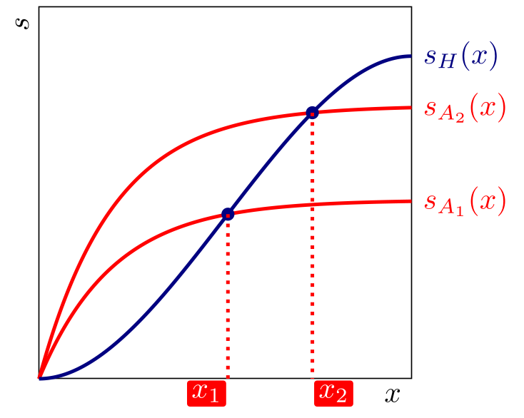
Unlike the fixed-budget metrics, this metric uses the agent’s entire performance curve, making it useful for tasks where we expect significant test-time scaling.

We define the “expenditure horizon” as the supremum of the common expenditures at which the agent matches or beats humans: $\sup\{x\geq 0:s_A(x)\geq s_H(x)\}$.

The expenditure horizon does not provide a finite crossing point if agents dominate humans at every level of expenditure.

Expenditure horizon can also be unstable if the slopes of $s_H$ and $s_A$ are similar.

Cunningham et al. (2026) introduce this metric, based in part on the apple-picking model (Cunningham and Shetty 2026).10

Human-Relative Expenditure Saving

image

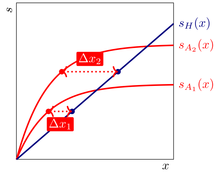
We can also directly measure the effective cost-saving relative to using a human on a task.

For simplicity we draw the human score curve as linear. We can then identify the point at which the marginal returns to expenditure are equal between agents and humans (assuming concave returns to expenditure on agents). If you are allocating budget between agents and humans then this will be the point at which you switch from spending on agents to spending on humans.

This point also identifies the economic value: the horizontal distance between the red and blue points represents the expenditure saving due to using an agent:

\[\Delta x_{A_i}=\max_{x\geq 0}\\{s_H^{-1}(s_{A_i}(x))-x\\}.\] This applies the utility framework discussed above, but now our indifference curves are determined by the returns to human labor (our outside option).

This is discussed further in Cunningham et al. (2026) and Cunningham and Shetty (2026).

Human-Relative Cost at Fixed Score

image

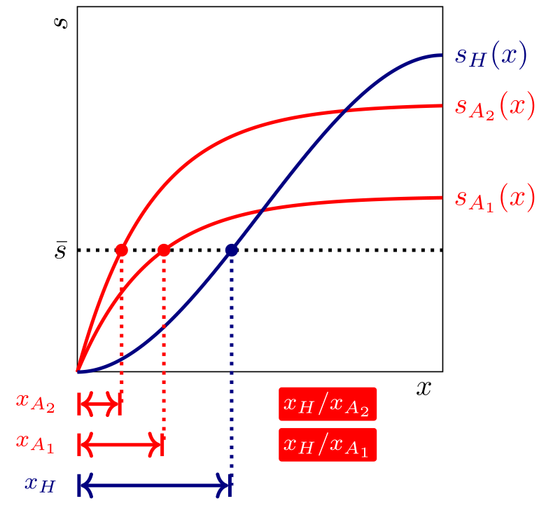
An alternative metric is to simply compare the cost of achieving some fixed score, $\bar{s}$. In the figure, $x_{A_i}=s_{A_i}^{-1}(\bar{s})$ and $x_H=s_H^{-1}(\bar{s})$:

\[\text{human-relative cost}_{A_i}(\bar{s})= \frac{s_H^{-1}(\bar{s})}{s_{A_i}^{-1}(\bar{s})} =\frac{x_H}{x_{A_i}}.\] This metric is consistent across values of $\bar{s}$ when the human and agent score curves differ only by a multiplicative horizontal rescaling.

Unlike the other metrics in this section, this metric remains useful when agents strictly dominate humans (i.e. the red curve is entirely to the left of the blue curve).

FAQ / Notes

Q: Can we interpret “score” as probability of success on a binary task? Many test-time scaling curves use $\Pr(\text{success})$ on the score axis. For example, OpenAI reports the probability of solving the Erdős unit-distance problem as test-time compute varies (OpenAI 2026). An important qualification is that, in applications where reliability has increasing marginal value, utility may be a convex function of the probability of success: going from 95% to 100% reliability can be far more valuable than going from 40% to 45%. We can transform $p$ into a reliability metric like $-\log_{10}(1-p)$, which measures orders-of-magnitude reductions in error—the “number of