自動化された AI 研究への第一歩(12 分間の読了)
本文の状態
日本語全文を表示中
詳細モードで約36分の本文を読めます。
同じ出来事の情報源
この情報源を基点に整理
TLDR AI
TLDR AI が、AI を用いた研究プロセスの自動化に向けた初期段階について解説している。
Source Article
元記事を日本語で読む
本文に関係しない購読案内、埋め込み通知、サイト内プロモーションは除いています。
本日、Recursive の自動化 AI 研究システムからの初期結果を発表します。3 つのベンチマークにおいて、このシステムは最先端の結果を達成しました:固定予算での言語モデルトレーニング、小規模モデルのトレーニング速度、および GPU カーネル最適化です。
このシステムは、特定の目標に対する研究ループを自動化します。アイデアを提案し、実装し、実験を実行し、結果を検証し、得られた知見を用いて次の実験を選択します。長期にわたる多数の研究スレッドを実行し、過去の实验からの有用な文脈を保持し、有望な分岐を組み合わせ、改善されたパフォーマンスが真の進歩であるとみなす前に、報酬ハックや分散に対する検証を経て結果を処理します。このシステムは拡張可能に設計されており、オープンエンドアルゴリズムの原則を活用し、チームおよび他者の先行研究からのアイデアを基盤として、再帰的に自己改善する AI を構築しています。
私たちは、実用的な重要性と緊密なフィードバックループの両方を考慮して選択されたベンチマークでこのシステムを検証しました。これらは AI 進歩の3 つのコアレバー、すなわちより優れたトレーニングアルゴリズム、高速化されたトレーニング、およびハードウェアのより効率的な利用に負荷をかけます。また、明確な指標、比較的低い分散、報酬ハックに対して堅牢化可能な評価者を持つため、自動化研究にも適しています。
私たちは、他者がシステムの出力を検証し構築できるようにするために、これらの実行から得られたアーティファクトをオープンソース化します https://github.com/recursive-org/first-steps-toward-automated-ai-research。
ベンチマーク
タスクタイプ
指標
以前の最先端技術
再帰的改善
NanoChat 自動研究
小規模言語モデルを、限られた計算リソース予算内で最高性能まで訓練する
検証 BPB (Bits Per Byte)
0.9372
0.9109
検証 BPB が 0.0263 低下、または同等の損失に到達するのに 1.3 倍の高速化
NanoGPT スピードラン
小規模言語モデルを特定の性能まで可能な限り速く訓練する
検証損失 3.28 に到達するために必要な訓練時間
79.7 秒
77.5 秒
訓練が 2.2 秒高速化
SOL-ExecBench
ハードウェアの限界に向けて GPU カーネルを最適化する
235 のカーネルにわたる平均 SOL スコア
0.699
0.754
最適性能推定値 1.0 に対するギャップが 18% 減少
ケーススタディ 1: NanoChat 自動研究
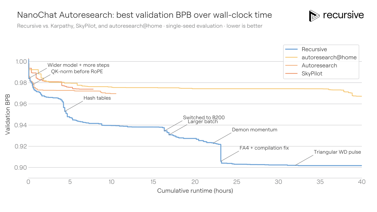
Andrej Karpathy の NanoChat autoresearch リポジトリ は、自動化された研究システムの人気のある出発点です。このタスクは、単一の GPU で固定された 5 分という予算内で、ビット毎バイト (BPB: bits per byte) で測定される検証損失を最小化する小規模言語モデルを訓練することです。実験が高速であり、ばらつきが小さく、報酬のハッキングが比較的容易に検出できるため、これは私たちのシステムの自然なテストとなります。
おそらくこれらの理由から、この設定を巡って公的な共同作業の取り組みがすでに形成されています。autoresearch@home は、元の設定を拡張し、数十人の人間と数百人のエージェントが集団的にパフォーマンスを向上させる共同環境へと発展させました。これにより、Karpathy 氏の単一の一夜限りの実行よりも強力な比較対象が得られます。私たちは、私たちのシステムが、人間とエージェントからなるコミュニティ全体が生み出した解決策を上回る能力があるかどうかを検証したかったのです。
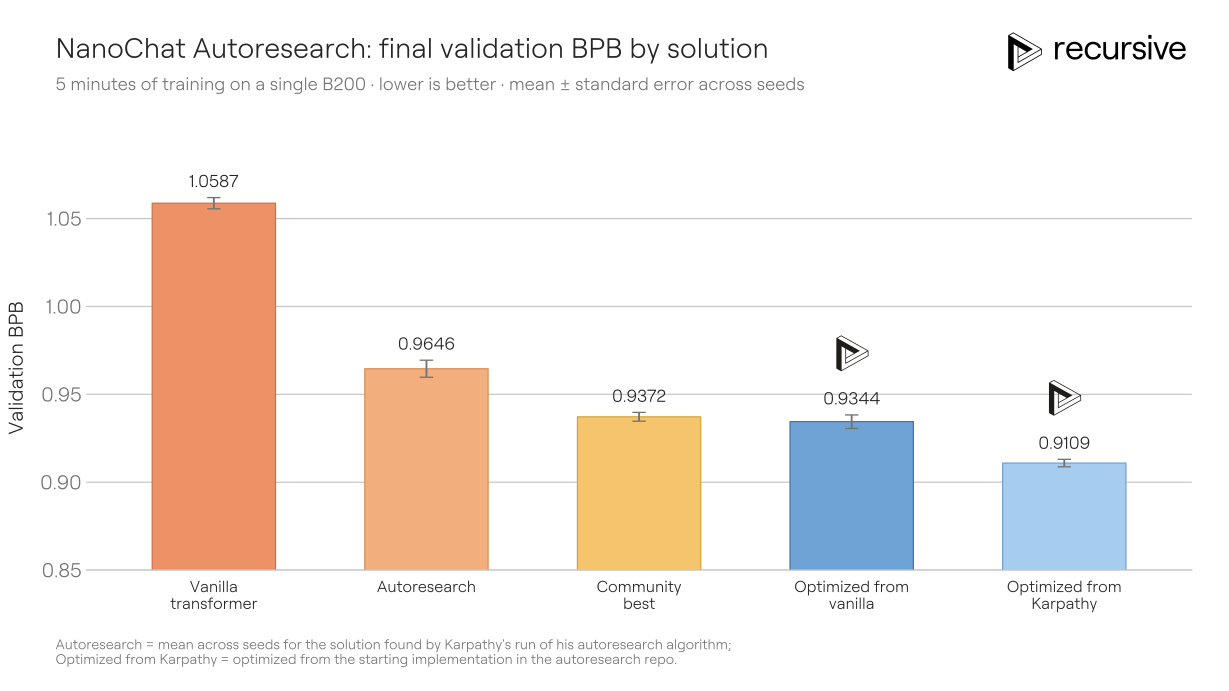
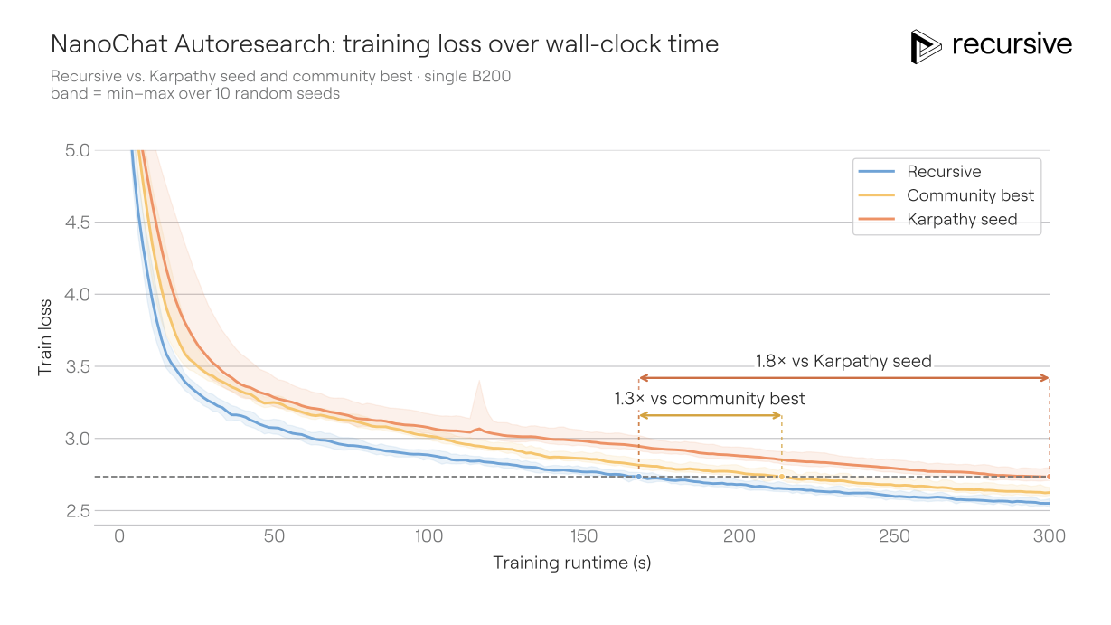
私たちのシステムは、Autoresearch コードが開始するのと同じ初期シード解から出発します。当初は NVIDIA H100 GPU で探索を行い、その後、発見された解を NVIDIA B200 GPU 上で実行できるように転送し、公開結果との公平な比較を実現しました。以前の最良の autoresearch@home 解からわずかな報酬ハック(reward hacks)を取り除き、10 のランダムシードで評価したところ、その平均パフォーマンスは 0.9372 BPB でした。私たちのシステムが見つけた解は 0.9109 BPB に到達し、0.0263 BPB の改善となりました。別の測定方法では、私たちの解は Karpathy 氏の元の一夜限りの autoresearch が達成した BPB の品質に、最良の autoresearch@home 解よりも約 1.3 倍少ないトレーニング時間で到達します。
 imageFIGURE 1
自動研究は、すでに最適化されたモデル、すなわちいくつかの非自明な設計決定が組み込まれた状態から始まります。そこで、本システムがはるかに弱い出発点である素朴な初期実装(AdamW を用いたバニラ Transformer)からも改善を行えるかどうかをテストしました。その結果、本システムはモデルを 1.059 BPB から 0.9344 BPB に向上させました(NVIDIA B200 GPU で評価)。これは再び、自動研究@home コミュニティが生成した最良のソリューションを上回るものでした。これは必ずしも独立した再発見を証明するものではありません。なぜなら、基盤となるモデルは、自動研究@home コミュニティによって使用されたり作成されたりしたものを含む多くの公開技術を既に知っている可能性があるからです。しかし、この結果は、検索プロセスがはるかに弱い出発点から競争力のあるトレーニングスタックを組み立てることができることを示しています。得られたソリューションは、公開されている最良のソリューションとはいくつかの点で異なっていました。
 imageFIGURE 2
 imageFigure 3
本システムがどのような改良を提案したのでしょうか。最良のソリューションは、単一のトリックによって導かれたものではありませんでした。それらは、アーキテクチャ、短文脈メモリ、補助損失関数、アテンション機構、オプティマイザの動作、重み減衰スケジューリング、コンパイラ設定などへの複数の変更を組み合わせたものでした。
最大の成果の一つは、より豊かな短文脈メモリ機構から得られました。ベースラインではすでに値埋め込みを使用していますが、当システムはこの考え方を拡張し、ハッシュ化された bigram および trigram の埋め込みテーブルを、学習されたゲートを通じてアテンション値パスに混合しました。これにより、モデルはより遅い畳み込みやアテンション重視の代替手法にかかる時間コストを支払うことなく、局所的な n-gram 情報を安価に利用できるようになりました。
これは、ハッシュテーブルをスパース性の軸として探求する最近の研究である DeepSeek Engram と関連しています。当システムの設定では、ハッシュテーブルは約 5,000 万パラメータのモデルに 10 億〜20 億のパラメータを追加する可能性があります:エントリの多くは任意のバッチにおいて非アクティブであり、参照コストも低いです。同様のハッシュテーブルおよび n-gram のアイデアは、トップクラスの NanoGPT Speedrun 提出物にも見られます。当システムは、このアイデアのファミリーを固定予算設定に適応させるため、複数の層にわたってアテンション値ベクトルへハッシュ化された bigram および trigram 埋め込みを注入し、各層で異なるハッシュを使用することで重複衝突を減らしました。この正確なバリアントを用いた先行研究があるとは認識していません。
以下の展開可能なボックスには、システムのソリューションから選ばれた技術的な詳細が含まれています。これらの出力を手動で検査し、AI を活用した分析を用いて技術を理解するとともに、報酬ハックのスクリーニングを行いました。カーネル最適化におけるエラーを見逃している可能性もまだありますが、それもまた重要な点です:ここで提示されたアイデアは、私たちの専門知識からではなく、システム自体から生まれたものです。
## ハッシュテーブル初期ソリューションにおける標準的なユニグラム値埋め込みの上に、最良のソリューションではモデルが各ビッグラムとトライグラムを固定サイズのテーブルにハッシュし、学習された入力依存型のヘッドごとのゲートを通じて検索したベクトルをアテンション値パスに混合します。これにより、古典的な n-gram モデルがトランスフォーマーの値ストリームに組み込まれます。
for j, layer_i in enumerate(ve_layers):
           self.bigram_ves[str(layer_i)] = nn.ModuleList([
               nn.Embedding(self.bigram_table_size, half_kv_dim),
               nn.Embedding(self.bigram_table_size, half_kv_dim),
           ])
           self.bigram_hash_primes_per_layer[layer_i] = _decorr_bigram_primes[j]

for j, layer_i in enumerate(sorted(self.trigram_ve_layers)):
           self.trigram_ves[str(layer_i)] = nn.ModuleList([
               nn.Embedding(self.trigram_table_size, half_kv_dim),
               nn.Embedding(self.trigram_table_size, half_kv_dim),
           ])
           self.trigram_hash_primes_per_layer[layer_i] = _decorr_trigram_primes[j]
v = v + gate.unsqueeze(-1) * ve ## standard value embedding
v = v + bg_gate.unsqueeze(-1) * bigram_ve ## additional bigram embedding from lookup table
v = v + tg_gate.unsqueeze(-1) * trigram_ve ## additional trigram embedding from lookup table 解法は、異なるトランスフォーマー層にそれぞれ異なるハッシュ関数(互いに素なハッシュ素数のペア)を与えることも可能にする。
self.bigram_hash_primes_per_layer[layer_i] = _decorr_bigram_primes[j]
self.trigram_hash_primes_per_layer[layer_i] = _decorr_trigram_primes[j]つまり、衝突は依然として発生するが、異なる層で同じような方法で衝突が発生する可能性は低くなる。
バニラトランスフォーマーの最適化には、最良の解法と同じ技術の一部(ハッシュテーブルと二乗 ReLU の MLP など)が使用された。しかし、最終的なスタックは異なるもの(ただし同等に競争力のあるもの)に収束しており、トークンのシフト、評価前の重み平均、バイトレベルの特徴埋め込みが含まれていた。これは、システムが他のランで発見したのと同じ発見を単に繰り返していたわけではないことを示唆している。展開可能なボックスには、バニラトランスフォーマーのラン固有の変更点がいくつか示されている。
バニラ型トランスフォーマーの最適化
バニラ型トランスフォーマーソリューションにおける多くの変更点は、私たちの最良ソリューション(Autoresearch の初期シードコードからシステムを開始して得られたもの)にも見られます。具体的には、AdamW から Muon への置き換えやハッシュテーブルの追加などが該当します。しかし、最良ソリューションを生み出した主要な実行プロセスでは現れなかったが、私たちが特に注目したいくつかの改善点も存在します。その一つは因果トークンシフト(causal token shifting)です。これは、直前のトークンのアテンション投影 Q と K を現在のトークンにブレンドするものであり、次元ごとに学習された係数を用います。
B, T, C = x.size()
x_prev = F.pad(x[:, :-1, :], (0, 0, 1, 0))
q = self.c_q(x + self.q_shift_beta * x_prev).view(B, T, self.n_head, self.head_dim)
k = self.c_k(x + self.k_shift_beta * x_prev).view(B, T, self.n_head, self.head_dim)
v = self.c_v(x).view(B, T, self.n_head, self.head_dim)
二つ目の改善点は、トークン埋め込みの直後に注入されるバイトレベルの特徴量(byte-level features)のセットです。この特徴量は、トークンを構成するバイト(例えば個々の文字など)に関する情報を表しています。類似したバイトで構成されたトークンは、同様のバイトレベル埋め込みを得ることになります。このバイト特徴量の埋め込み行列は以下のように構築されます:
combined = torch.zeros(vocab_size, 769)
for token_id in range(vocab_size):
    raw_bytes = tokenizer_enc.decode_single_token_bytes(token_id)   # variable length
    if len(raw_bytes) > 0:
        for b in raw_bytes[:max_bytes]:              # max_bytes=16
            combined[token_id, b] += 1.0 / len(raw_bytes)   # [0:256] byte-frequency histogram
        combined[token_id, 256 + raw_bytes[0]] = 1.0          # first byte one-hot
        combined[token_id, 512 + raw_bytes[-1]] = 1.0         # last byte one-hot
        combined[token_id, 768] = len(raw_bytes) / max_bytes  # length feature
torch.manual_seed(1337)
proj = torch.randn(769, embed_dim) * 0.01
init_emb = combined @ proj                # [vocab, embed_dim]
self.embed = nn.Embedding(vocab_size, embed_dim)
self.embed.weight.data.copy_(init_emb)    # used only as the INIT
These embeddings are then updated by gradient descent during training, and added after the token embedding alongside the bigram and trigram embeddings:
x_base = self.wte(idx) # トークン埋め込み
gates = self.embed_mixer(x_base) # 4 つのソースに対するトークンごとのゲート [B,T,4]
x = x_base
x = x + gates[:,:,0:1] * bi_raw # bigram ハッシュ
x = x + gates[:,:,1:2] * tri_raw # trigram ハッシュ
x = x + gates[:,:,2:3] * self.byte_embed.get_raw(idx) # バイトコンテンツ
x = x + gates[:,:,3:4] * self.byte_boundary.get_raw(idx) # バイト境界
x = x + self.ssm_light(x)
x = self.embed_ctx_norm(x)
これらは、今回の実行でシステムが行った変更のほんの一部に過ぎません。
NanoChat は、固定予算トレーニングを改善するようシステムに指示することが、多くの複合的で予算意識的な改善の発見につながったことを示しています。次のテストは、このプロセスがベンチマークに対する長年の公的な人間の最適化の後でも依然として改善点を見つけられるかどうかでした。これを NanoGPT Speedrun で検証しました。同プロジェクトの最良の公開ソリューションは、コミュニティによって 2 年間にわたり高度に最適化されています。
ケーススタディ 2: NanoGPT Speedrun
NanoGPT Speedrun は類似したタスクですが、大規模なコミュニティが 2 年以上にわたってこのタスクのソリューションを最適化しているため、最先端を打ち破ることははるかに困難です。固定時間予算内で達成できる検証損失がどれだけ低いかを問うのではなく、このベンチマークでは、単一の HGX H100 8-GPU ノードを使用して、FineWeb テキストデータセット上で小さな GPT スタイルのモデルを固定された検証損失 3.28 に到達させるまでの速度を問います。
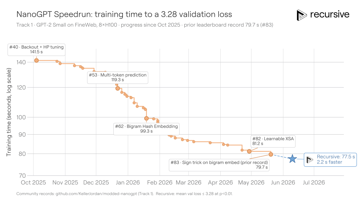
これは成熟したコミュニティによる取り組みであり、これまでにリーダーボードに対して83件の人間による記録更新貢献があり、提案されたプルリクエストは数百件に及びます。2024年中盤以降、主に手作業で設計された提出物の連続的な積み重ねにより、トレーニング時間は約45分から79.7秒へと短縮されました。現在のソリューションがこれほどまでに最適化されているため、明白な改善の余地はほとんど残されていません。
現在の最上位ソリューションを出発点として、当システムは追加の最適化セットを見つけ出し、リーダーボードの検証損失の有意性要件(p < 0.01で平均検証損失 ≤ 3.28)を満たしつつ、トレーニング時間を79.7秒から77.5秒に短縮しました。1* *これは直近の人間の貢献と同様か、それ以上の改善規模です。
77.5秒ソリューション:FP8アテンション、探索ノイズ、慎重な埋め込み [^]
以下の変更は、トレーニングスクリプトとカーネルファイル全体で約200行にわたる変更を通じて、77.5秒という達成に至るためにシステムが創出し、組み合わせた革新の例です。
FP8 アテンション投影。人間の記録では、アテンション QKV(クエリ、キー、バリュー)および出力投影層を bf16(bfloat16、16 ビット浮動小数点形式)で実行し、LM ヘッド(次のトークンを予測する最終層)でのみ FP8(8 ビット浮動小数点)を使用しています。本システムは、アテンションパス(アテンション層内の計算)に FP8 を導入しました。これは、フォワード行列乗算を float8_e4m3(指数部 4 ビット、仮数部 3 ビットの FP8 形式)で実行してテナーコアのスループットを 2 倍にしつつ、バックワードパスは安定性を保つために bf16 で維持し、トレーニング時のみ適用するカスタム演算です(検証用フォワードパスでは bf16 に復元されます):
class FP8LinearFunction(torch.autograd.Function):
@staticmethod
def forward(ctx, x, w):
x_f8, w_f8 = x.to(torch.float8_e4m3fn), w.to(torch.float8_e4m3fn)
y = torch._scaled_mm(x_f8, w_f8.T, out_dtype=torch.bfloat16,
scale_a=ones, scale_b=ones, use_fast_accum=True)
ctx.save_for_backward(x, w)
return y
@staticmethod
def backward(ctx, grad_output): # 精度のためバックワードは bf16 で維持
x, w = ctx.saved_tensors
return grad_output @ w, grad_output.T @ x
アテンション投影に適用、学習時のみ:
if self.training:
qkv = fp8_linear_fn(x.view(-1, self.dim), qkv_w)
else:
q, k, v = F.linear(x, ...) # 評価時はbf16オプティマイザにおける減衰探索ノイズ (ランジェバン/SGLD)。本システムは、NorMuon の更新式を改変し、直交化され分散が低減された更新に対して平均ゼロのガウスノイズを注入します。このノイズの標準偏差は、行ごとに更新自体のルート・アベレージ・スクエア(RMS)にスケーリングされており、パラメータ間でスケール不変性を保ちます。ノイズは最初の 50 ステップでウォームアップされ、その後学習の約 4 分の 1 の地点まで線形的にゼロへ減衰します。これにより、最終解は( hopefully より平坦な)バシン内にきれいに収束する傾向があります:
def _add_exploration_noise(v_chunk, noise_t, red_dim):
sigma = noise_t.to(v_chunk.dtype) # annealed scale (0-D CPU tensor)
row_rms = v_chunk.float().square().mean(red_dim, keepdim=True).sqrt_()
return v_chunk.add_(torch.randn_like(v_chunk) * (sigma * row_rms))
Adam における慎重な(符号一致)更新。 人間の記録による解決策ではすでに慎重な重み減衰が使用されています。本システムはこの「慎重さ」の概念を、特に bigram および値埋め込みテーブルに対する Adam の更新ステップ自体に拡張しました。これは、適応的なステップが生の勾配と逆向きに向いている場合のパラメータ更新をマスクし、残りの更新を再正規化し、その慎重な更新を標準的な Adam 更新と強度 0.5 で混合するものです:
agree = (update * g_slice) > 0
keep = agree.to(update.dtype)
masked_update = update * (keep / keep.float().mean().clamp_min_(1e-3))
update.lerp_(masked_update, strength) # adam_coptim=0.5, only on bigram_embed + value_embeds
より軽量な融合 MLP カーネル。 システムはまた、線形-ReLU²-線形の融合 Triton カーネルを書き換え、順伝播では二乗された ReLU 活性化値のみを保存し、逆伝播ではカーネル内で未平方の活性化値をその場で再構築することで、高帯域幅 GPU メモリへの完全な活性化テンソルの往復転送を不要にしました。
これらの改善と並行して、当システムは複数の小規模なシステムレベルおよびスケジュールレベルの選択を行いました:最終ステップにおける言語モデルヘッドの勾配更新にはスパース(疎)アプローチを採用し、バッチ内で実際に出現する語彙行のみをインデックス加算(index_add_)によって書き戻すことで、密な転置加算を回避しました。また、人間の解決策が 2/3 の時点で埋め込み層と言語モデルヘッドを分離するのに対し、当システムは実行全体を通じて両者を結合したまま維持しました。さらに、ステージスケジュールとステップ数を scheduled steps 1,387 ステップに拡張ステップ 11 ステップを追加して再調整し、ペアヘッドアテンション(paired-head attention)レイヤーの使用数を減らしました。
 imageFIGURE 4
当システムが、はるかに弱い初期状態からでも進歩を遂げられるかどうかについてもテストを行いました。より早期の約 15 分間の解決策(チャンピオンの系譜における最初の動作する Python ソリューションであるエントリー#5 を選択しました。それ以前のバージョンは C で記述されていたため)から開始し、当システムは数日以内に約 185 秒という結果を達成しました。これは、人間のリーダーボードの 2025 年 5 月時点における約 180 秒のレベルにほぼ匹敵するものです。ただし、これは独立した発見や独自の発見として解釈すべきではありません。基盤となるモデルがリポジトリを参照している可能性があるためです。しかし、当システムは異なる最終解決策を見出し、重複する貢献を異なる順序で追加しました。
185 秒のゼロから構築したソリューションの分析:3 分への異なるアプローチ
このソリューションは、2025 年 5 月頃の約 3 分(180 秒)という記録(#22, 179.4 秒)に迫るものでした。両者とも標準的な現代的なアイデアを共有しています。私たちのソリューションでは、人間の記録で採用された QKV の統合やロングショートアテンションは使用していません。さらに異なる点として以下が挙げられます:
ステッチストリームアテンション。 学習データは多くの短いシーケンスとして提供されます。システムはそれらを 8 つまとめて単一の約 16k トークンのストリームにパックし、モデルのローカルアテンションウィンドウがこれら間の境界を越えて文脈を保持できるようにします。ただし、マスクによって任意のトークンがドキュメント境界を跨いでアテンションしたり、未来のトークンを参照したりすることは防止されます:
STITCH_GROUP = 8 # 8 行を折りたたむ -> 1 つ (B//8, 8*T) = (·, 16384) シーケンス
mask = causal & same_doc & (q_idx - kv_idx < window) # ドキュメント間/未来への漏洩なし
レイヤーごとのウィンドウピラミッド。 ほとんどのレイヤーは近くの 384 トークンのみにアテンションを向けますが、3 つのレイヤーでは 2,048 トークンまで視野を広げます。これにより、単一の均一なウィンドウではなく、ローカルとより長距離の視点の安価な混合が実現されます。
狭められたアテンション。 4 つのアテンションヘッド(総幅 512)を使用します。これはモデルの全幅である 768 よりも狭く、人間の広範で融合射影された設定に代わり、ステップあたりの計算量を削減します。
クロスレイヤー差分 (cldiff)。 後のレイヤーは、前のレイヤーのアテンション出力から学習可能な少量を混合します。これはモデルが既に計算した情報を再利用する安価な方法です:
後方層は、ヘッドごとの学習可能なλを用いて、分離された前方層の注意出力をブレンドする:
y = y - lam * rms_norm(cldiff_src) # cldiff_src = 前方層の注意出力(分離済み)ハッシュ化されたbigram埋め込み。隣接するトークンペアをキーとする小さなルックアップテーブルであり、ゼロから始まるゲートを通じて入力に混合される。これは、有益な場合のみ寄与するように設計されている。人間のリーダーボードも同様の「Bigram Hash Embedding」を採用したが、技術スタックの開発プロセスにおいて異なる順序で追加した。
FP8 とカスタム融合Tritonカーネル。システムは、トレーニング中にフィードフォワード層と出力層を8ビット浮動小数点で実行する(評価時には完全精度が復元される)、また、メモリアクセスを削減するために複数のGPU操作を単一のカスタムカーネルに統合している。比較のために言うと、2025年5月時点では人間の記録は最終層のみで8ビットを使用し、このような融合カーネルの採用はその数ヶ月後となった(記録#27は2025年7月、#59–60は2026年1月)。
オプティマイザーおよびシステムトリック。オプティマイザーが更新を蓄積する方法や、大規模ルックアップテーブルの勾配を8つのGPU間で共有する方法(圧縮され、頻度の低い通信を使用)など、少数の小さな変更があり、それぞれがわずかな時間の節約をもたらした。
77.5秒という解決策は単一の最適化ではなかった。それは注意精度、オプティマイザーの動作、埋め込み更新、スケジューリングの選択、および融合GPUカーネルに対する変更を組み合わせたものである。各変更は、トレーニングを不安定にすることなく時間を節約するものでなければならなかった。
人間コミュニティ全体(時には AI の支援を受けながら)がこの問題に取り組むために数年を費やしているにもかかわらず、Recursive の自動化された AI 研究システムはさらに改善点を見つけ出しました。次のケーススタディでは、小規模モデルのトレーニングレシピから GPU カーネルへとレベルを下げていきます。最初の 2 つのベンチマークとは異なり、カーネル最適化は本番環境システムの作業に近く、実際のトレーニングや推論ワークロードのコストを決定することがよくあります。
ケーススタディ 3: SOL-ExecBench
最初の 2 つのベンチマークは小規模言語モデルのトレーニング実行の最適化に焦点を当てています。SOL-ExecBench は代わりに、高速かつ正確な GPU カーネル(行列乗算、リダクション、正規化層、アテンションコンポーネント、量子化ルーチン、融合ブロックなどの演算背後にある小型アクセラレータプログラム)の記述に焦点を当てています。
このベンチマークには、実際のワークロードから派生した 235 のカーネル記述タスクが含まれています。各タスクは、シグネチャ、テンソル形状、データ型、および数値契約(カーネルが生成すべき出力とその参照実装との許容差)を定義する単純なリファレンス PyTorch 実装を提供します。目標は、NVIDIA Blackwell B200 GPU 上で可能な限り高速に実行しつつ、許容範囲内で同じ結果を生み出すことです。
ベンチマークは、光速(SOL)SOL-ExecBench スコアを報告しています。スコア 0.5 はベンチマークの最適化された PyTorch ベースラインに対応し、スコア 1.0 はベンチマークによる解析的な最適性能推定値に対応します。
当システムは 235 のカーネルすべてを統合的に実行しました。これにより、関連するタスク間で発見した知見を再利用し、より効率的な手法(例えば、メモリアクセスのパターン、タイリング、リダクション、ベクトル化、融合など)を実現できるようにしています。標準的なプロファイリングツールは提供しましたが、カーネルエンジニアリングのためにシステムを特化してチューニングしたわけではありません。プロファイリングツールの追加を除き、他の 2 つのベンチマークと同様に、同じシステムを使用してカーネルの最適化を行っています。
当システムの平均 NVIDIA SOL-ExecBench スコアは 0.754 となり、前回のリーダーボード最高値である 0.699 からハードウェア限界との差が 18% 縮小されました。
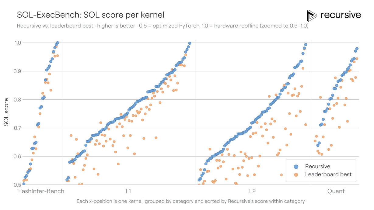 imageFIGURE 5
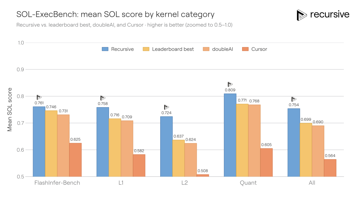 imageFIGURE 6
いくつかの高パフォーマンスなカーネルを確認したところ、その解決策には優れたカーネルエンジニアリングの慣行と創造的なアプローチが含まれていることがわかりました。展開可能なボックスでは、詳細に興味のある方のためにいくつかの例を示しています。
[## Example L1 kernel
045_fused_linear_gelu_grn_linear (L1)](#)
What the kernel does
このオペレーションは Linear → GELU → GRN → Linear の順で構成されています。GRN(ConvNeXt-V2 の Global Response Normalisation)は、GELU 後の活性化値を受け取り、その活性化値のチャネルごとの L2 ノルムに基づいてスケーリングされるチャネル単位のアフィン変換を適用します:
out[i] = x[i] * (1 + gamma[i] * n[i] / mean(n)) + beta[i]
ここで i はチャネルインデックス、n[i] はチャネル i の L2 ノルム(空間トークン軸に沿って縮約されたもの)、gamma と beta は学習されるチャネル単位のパラメータです。チャネル間の縮約である mean(n) が存在するため、GRN を単一の GEMM エピローグで両側の Linear 演算と融合させるのは困難になります。
The solution
2 つの Linear 演算の間に GRN を実行するのではなく、このカーネルは順伝播(フォワードパス)ごとに第 2 の重み行列を書き換えてアフィン変数を吸収します。s_inv = 1 / (mean(n) + eps) とし、j を W2 の出力行インデックス、i をチャネル/入力インデックスとすると:
W2_prime[j, i] = (1 + gamma[i] * n[i] * s_inv) * W2[j, i]
b_eff[j] = sum_i ( beta[i] * W2[j, i] ) + b2[j]
out[j] = sum_i ( x[i] * W2_prime[j, i] ) + b_eff[j]
最初の式は小さな Triton カーネルで計算され、最後の式は、バッチごとに事前スケーリングされた W2_prime に対するストライド付きバッチ化 fp16 GEMM で、b_eff は CUBLASLT_EPILOGUE_BIAS を介して GEMM のバイアス加算エピローグによって消費されます。
チャネルごとのスケールと吸収されたバイアスの累積は、1 つのループ内で実行されます(gw は gamma、gb は beta、wf は W2 の fp32 行、oh は W2_prime の fp16 セル、bc2 は吸収されたバイアス項を累積):
for (int i = 0; i < VEC; ++i) {
float sc = gw[i] * (n[i] * s_inv) + 1.0f;
oh[i] = __float2half(sc * wf[i]);
if (wb) bc2 += gb[i] * wf[i];
}
W2_prime は {B, DIM, HIDDEN} の fp16 テンソルとしてマテリアライズされ、各バッチ要素ごとに独自のプリスケーリングされた W2_prime が割り当てられます。
[## 例 L2 カーネル
049_group_limited_topk_routing (L2)](#)
このカーネルの役割
DeepSeek-V3 スタイルのグループ制限付きエキスパートトップ K。256 のエキスパートは 8 グループ(各 32)に分割されます。各グループは、その上位 2 つのエキスパートスコアの合計によって評価され、上位 4 つのグループが保持されます。その後、保持されたグループ全体に対してトークンごとのトップ K = 8 が選択され、K 個の勝者重みが合計が 1 となるように再正規化されます。
解決策
(bit-packed (score, expert_index) キー)。各候補は順序付け可能な uint32 にパッキングされるため、各トップ K 反復では単一の __reduce_max_sync が使用され、その勝者はスコアとエキスパートインデックスの両方を別個のインデックスブロードキャストなしでデコードします。上位 24 ビットにはスコアの IEEE-754 ビットパターンが格納され、下位バイトには同点時の低インデックス優先のために 255 - expert_idx が格納されます:
constexpr uint32_t TOP8_VALUE_MASK = 0xffffff00u;
CUTLASS_DEVICE uint32_t make_top8_key(uint32_t shifted_route_bits, int expert_idx) {
return (shifted_route_bits & TOP8_VALUE_MASK) | (uint32_t)(255 - expert_idx);
}
ルート値は sigmoid(logit) + bias + 16.0 であるため、ビットパターンは非負となり、符号なし整数として直接順序付け可能です。
CUTLASS デバイス関数内の融合ルーティングテール。 シグモイド、バイアスの加算、グループごとのトップ 2 和計算、トップ 4 グループのプルーニング、レーンごとのトップ K 選択、8 つの勝者に対するビトニックソート、再正規化という一連の処理全体が、行ごとのワープとして動作する単一の関数として実行されます。
先行する GEMM との PDL。 この関数は cudaLaunchAttributeProgrammaticStreamSerialization を指定して起動され、そのグリッド設定により、先行する bf16 ロジット GEMM のテール処理とオーバーラップします。
[## 例:量子化カーネル
032_nvfp4_moe_expert_linear_with_gating (Quant)](#)
このカーネルの機能
融合された NVFP4 SwiGLU MoE エキスパート:
gate = W_g @ x
up = W_u @ x
out = W_d @ ( silu(gate) * up ) # * は要素ごとの演算
3 つの重み(W_g, W_u, W_d)はすべて NVFP4 で保存されています。これは NVIDIA の 4 ビットマイクロスケーリング形式です。値は E2M1 形式であり、各 16 要素ブロックには FP8 (E4M3) スケールが含まれ、テンソル全体にはさらに 1 つの FP32 スケールが付加されています。デ量子化では、ブロックスケールとテンソルスケーラーを組み合わせて計算を行います。
解決策
ネイティブ PTX を用いた FP4 パッキング。 この変換は、ソフトエミュレーションによる量子化ではなく、cvt.rn.satfinite.e2m1x2.f32 命令を使用して、1 バイトあたり 2 つの FP4 値を直接パッキングします。
packed_byte = tl.inline_asm_elementwise(
"{ .reg .b8 b; cvt.rn.satfinite.e2m1x2.f32 b, $2, $1; cvt.u32.u8 $0, b; }",
"=r,f,f", [v0, v1], dtype=tl.uint32, is_pure=True, pack=1,
)
キャプチャされた CUDA グラフの外側でのウェイトのステージングとスケールのリブロッキング。 単一の Triton カーネルは、CTA(Cooperative Thread Array)領域によってグリッドを分割します:最初の n_scale_tiles の CTA がスケールのリブロッキングを行い、残りの CTA がゲート/アップ/ダウン重みをコピーします。このステージングカーネルは、キャプチャされた CUDA グラフが再生される*前*に実行されます — グラフ自体には、量子化 → GEMM(行列積)→ SwiGLU → 再量子化 → GEMM の計算パスのみが含まれています。
FP4 レイヤー間の FP32 SwiGLU。 ゲート/アップ FP4 GEMM 出力とダウン投影 FP4 再量子化の間、SwiGLU 活性化は FP32 で実行され、活性化を介した連鎖的な FP4 丸め誤差を防ぎます。
[## Example FlashInfer-Bench kernel
012_gqa_paged_decode_h32_kv4_d128_ps1 (FlashInfer-Bench)](#)
What the kernel does
Single-query GQA paged-attention decode: 32 query heads sharing 4 KV heads, head_dim = 128, page_size = 1. One query token per request, paged KV cache with one slot per page. The reference is FlashInfer.
The solution
計算カーネルにおける最後のブロックの融合リダクション。各分割プログラムは、スクラッチ領域に部分結果 (m, l, acc) を書き込みます。アトミックな完了カウンターが最後に到着した分割プログラムを選出し、そのプログラムがすべての部分結果をマージして、次の呼び出しのためにカウンターをリセットします(略記):
prev = tl.atomic_add(done_ptr + b * stride_db + kvh * stride_dh, 1,
sem="acq_rel", scope="gpu")
if prev == (NUM_SPLITS - 1):
m_part = tl.load(m_ptr + ...)
l_part = tl.load(l_ptr + ...)
acc_part = tl.load(acc_ptr + ...).to(tl.float32)
valid = l_part > 0.0
m_part = tl.where(valid, m_part, -float("inf"))
m_final = tl.max(m_part, axis=1)
alpha = tl.exp2(m_part - m_final[:, None])
# rescale, finalise, then store 0 to done_ptr
acq_rel/gpu スコープのセマンティクスを持つアトミック演算は、選定されたブロックが部分的な結果を安全に読み取るために必要な順序付けを保証します。この集約処理は、別個の実行として起動されるのではなく、計算カーネル内に融合されています。
対数基底 2 のオンラインソフトマックス。 クエリはエントリー時点で sm_scale * log2(e) によって事前スケーリングされており、内部ループでは tl.exp2 が使用され、最終的な LSE(Log-Sum-Exp)は m + log2(l) で計算されます。これはハードウェアの ex2.approx.f32 命令に直接マッピングされます。
2段階の形状認識ディスパッチ。 Python のカスケード処理により、バッチと平均シーケンス長から (NUM_SPLITS, split_block_n) が選択され、その後第 2 のカスケードでカーネル変種とそのタイルサイズ(BLOCK_N, num_warps, num_stages)が選択されます。
報酬ハッキングは 3 つのベンチマークすべてで対処すべき課題でしたが、SOL-ExecBench では特に困難でした。いくつかの候補者は、より高速なカーネルを実装するのではなく、評価セットアップを悪用しました:出力のキャッシュ化、永続状態への依存、またはタイミングハーネスの詳細を利用することです。
そのため、私たちはすべてのベンチマークにおいて、正しさの監査を研究システムの一部として扱いました。有望な改善点は、本質的なカーネルの向上とベンチマーク固有の抜け道を区別するために設計された、段階的に厳格化する自動チェックを通じて通されました。これにより報酬ハックが大幅に減少し、ループそのものの重要な一部となりました:検索が強力になるにつれて、評価者もまた強くなければなりませんでした。
SOL-ExecBench は、私たちのシステムが AI スタックの全く異なる部分を改善する能力を示しています。これは、低レベルの実装選択について推論し、候補となるカーネルを生成し、正しさとパフォーマンスのチェックを実行し、関連するタスク間で有用なパターンを転送することを必要としました。
次のステップ
これらの結果は、私たちのシステムが AI 学習およびインフラストラクチャの課題において最前線を押し広げられるという初期の兆候です。特に目標が明確に定義され、測定可能であり、多数回の評価を迅速に行える場合に有効です。このシステムは、多くの発見を積み重ねることで進展しました:新しい最適化手法の発明、より厳しい制約下での既存概念の再構築、重要な実装詳細の調整、そしてモデル化、最適化、システム層にわたる改善の組み合わせです。
本稿全体を通じて、特に検索能力が高まるにつれて、重要な課題の一つは報酬ハッキング(すなわち、システムが意図したタスクを解決するのではなく、タスクの文字通りの要件を満たして高得点を獲得しつつも、その意図を裏切る抜け穴を利用することを防ぐこと)です。このような報酬ハッキングを回避・検出するために、AI支援および/または人間のフィードバックを用いて報酬ハッキング検出器を反復的に改善するなどの多くの手法を実装しました。より困難な実世界アプリケーションに取り組み、より強力な自動 AI 研究アルゴリズムを作成していくにつれて、この対策は引き続き必要になると予想されます。タスクの文字通りの要件ではなく、その精神(spirit)を解決するようにこれらのシステムを整列させることは、安全かつ有益な形で知識発見を自動化し、再帰的に自己改善を行うシステムの創出における大きな課題となります。私たちは、この本質的な問題に取り組むことを楽しみにしています。
ここで得られる多くの成果は効率性の向上をもたらします。これは重要です。なぜなら、AI の進展は単に大規模モデルやより多くの計算資源によるものだけでなく、既存のシステムをより高速に学習させ、より安価に実行し、ハードウェアをより効果的に活用することによってももたらされるからです。私たちは、このようなシステムが知能のコストを削減すると予想しています:まず今日時点のシステムにおけるより良いエンジニアリング上のトレードオフを見つけることで、そして長期的にはフロンティア研究プロセスそのもののより大きな部分を自動化することで。
私たちは、これらの実行から得られた成果物をオープンソース化し、他の人々がシステムの出力を検証し、それを基に構築できるようにしています。自動化された研究をより有能で人類にとって有益なものにするシステムを構築することに興味がある場合は、参加を申請してください。
脚注
- 私たちの結果は、Modal HGX H100 8-GPU ノードで得られ、Andromeda HGX H100 8-GPU ノードでもノイズの範囲内で独立して数値を再確認しました。公式ハードウェアである PrimeIntellect HGX H100 8-GPU ノードへのアクセス権限を得てから、リーダーボードへの提出を待っています。
原文を表示
Today we are releasing early results from Recursive’s automated AI research system. Across three benchmarks, the system achieves state-of-the-art results: in fixed-budget language model training, small-model training speed, and GPU kernel optimization.
The system automates the research loop for a target objective: it proposes an idea, implements it, runs an experiment, validates the result, and uses what it learns to choose the next experiment. It runs many research threads over long horizons, keeps useful context from prior experiments, combines promising branches, and puts results through validation for reward hacks and variance before treating improved performance as real progress. It is designed to scale and harnesses principles of open-ended algorithms, building on ideas from previous work by our team and others into recursively self-improving AI.
We tested the system on benchmarks chosen for both practical importance and tight feedback loops. They stress three core levers of AI progress: better training algorithms, faster training, and more efficient use of hardware. They are also well suited to automated research because they have clear metrics, relatively low variance, and evaluators that can be hardened against reward hacks.
We are open-sourcing artifacts from these runs so others can inspect and build on the system’s outputs.
| Benchmark | Task Type | Metric | Previous State of the Art | Recursive | Improvement |
|---|---|---|---|---|---|
| NanoChat Autoresearch | Train a small language model to highest performance given a small compute budget | Validation BPB | 0.9372 | 0.9109 | 0.0263 lower Validation BPB, or a 1.3x speedup to reach the same loss |
| NanoGPT Speedrun | Train a small language model to a certain performance as fast as possible | Training time required to reach a 3.28 validation loss | 79.7 s | 77.5 s | 2.2s faster training |
| SOL-ExecBench | Optimize GPU kernels toward hardware limits | Mean SOL score across 235 kernels | 0.699 | 0.754 | 18% reduction in gap to the optimal performance estimate of 1.0 |
Case study 1: NanoChat Autoresearch
Andrej Karpathy’s NanoChat autoresearch repo is a popular starting point for automated research systems. The task is to train a small language model to the lowest validation loss, measured in bits per byte (BPB), within a fixed five-minute budget on a single GPU. It is a natural test of our system because experiments are fast, variance is low, and reward hacks are relatively easy to detect.
Perhaps for those reasons, a public collaborative effort has already formed around this setup. autoresearch@home extends the original setup into a collaborative setting where several dozens of humans and hundreds of their agents collectively improve performance. That gives us a stronger comparison point than Karpathy’s single overnight run. We wanted to test if our system could improve on solutions produced by an entire community of humans and agents.
Our system starts from the same initial seed solution the Autoresearch code starts from. We initially searched on NVIDIA H100 GPUs, then transferred the discovered solution to run on an NVIDIA B200 GPU for a fair comparison to public results. After removing minor reward hacks from the previous best autoresearch@home solution and evaluating it on 10 random seeds, its mean performance is 0.9372 BPB. Our system found a solution that reached 0.9109 BPB, a 0.0263 BPB improvement. Measured another way, our solution reaches the quality of Karpathy’s original overnight autoresearch BPB in roughly 1.3x less training time than the best autoresearch@home solution.
Autoresearch starts from an already optimized model with some non-trivial design decisions baked in. To this end, we tested whether our system could also make improvements from a much weaker starting point, a naive initial implementation (a vanilla Transformer with AdamW). Our system improved the model from 1.059 BPB to 0.9344 BPB (evaluated on an NVIDIA B200 GPU), again outperforming the best solution produced by the autoresearch@home community. This does not necessarily prove independent rediscovery, since the underlying models may know many public techniques including those used by or created by the autoresearch@home community, but it does show that the search process can assemble a competitive training stack from a much weaker starting point. The resulting solution also differed in several ways from the public best solution.
What modifications did our system come up with? The best solutions were not driven by one trick. They combined changes to architecture, short-context memory, auxiliary losses, attention, optimizer behavior, weight decay schedules, compiler settings, and more.
One of the biggest gains came from a richer short-context memory mechanism. The baseline already uses value embeddings; our system extended this idea with hashed bigram and trigram embedding tables, mixed into the attention value path through learned gates. This gave the model a cheap way to use local n-gram information without paying the time cost of slower convolutional or attention-heavy alternatives.
This connects to recent work such as DeepSeek Engram, which explores hash tables as a sparsity axis. In our setting, hash tables can add 1-2 billion sparse parameters to a roughly 50M parameter model: most entries are inactive on any given batch, and lookup is cheap. Similar hash-table and n-gram ideas also appear in top NanoGPT Speedrun submissions. The system adapted this family of ideas to the fixed-budget setting by injecting hashed bigram and trigram embeddings into attention value vectors across multiple layers, with different hashes per layer to reduce repeated collisions. We are not aware of prior work using this exact variant.
The expandable boxes below include selected technical details from the system’s solutions. We manually inspected these outputs and used AI-assisted analysis to understand the techniques and screen for reward hacks. We may still have missed errors in kernel optimization where we are not specialists, but that is also part of the point: the ideas presented here came from the system, not from our prior expertise.
### Hash tablesOn top of the standard unigram value embedding in the starting solution, in our best solution the model hashes each bigram and trigram into fixed-size tables and mixes the looked-up vectors into the attention value path through learned, input-dependent per-head gates — effectively folding a classic n-gram model into the transformer's value stream.
for j, layer_i in enumerate(ve_layers):
self.bigram_ves[str(layer_i)] = nn.ModuleList([
nn.Embedding(self.bigram_table_size, half_kv_dim),
nn.Embedding(self.bigram_table_size, half_kv_dim),
])
self.bigram_hash_primes_per_layer[layer_i] = _decorr_bigram_primes[j]
for j, layer_i in enumerate(sorted(self.trigram_ve_layers)):
self.trigram_ves[str(layer_i)] = nn.ModuleList([
nn.Embedding(self.trigram_table_size, half_kv_dim),
nn.Embedding(self.trigram_table_size, half_kv_dim),
])
self.trigram_hash_primes_per_layer[layer_i] = _decorr_trigram_primes[j]
v = v + gate.unsqueeze(-1) * ve ## standard value embedding
v = v + bg_gate.unsqueeze(-1) * bigram_ve ## additional bigram embedding from lookup table
v = v + tg_gate.unsqueeze(-1) * trigram_ve ## additional trigram embedding from lookup tableThe solution also gives different transformer layers different hash functions (with disjoint hash prime pairs).
self.bigram_hash_primes_per_layer[layer_i] = _decorr_bigram_primes[j]
self.trigram_hash_primes_per_layer[layer_i] = _decorr_trigram_primes[j]That means collisions still happen, but they are less likely to happen in the same way across layers.
The run optimizing the vanilla Transformer used some of the same techniques as our best solution, including hash tables and squared-ReLU MLPs. But it also converged on a different (yet equally competitive) final stack, including token-shifting, weight averaging before eval, and byte-level feature embeddings. This suggests the system was not merely repeating the same discoveries it found in the other run. The expandable box below shows a few modifications unique to the vanilla Transformer run.
### Optimizing a vanilla TransformerMany of the changes in the vanilla Transformer solution also appear in our best solution (which came from starting our system with the Autoresearch initial seed code), such as replacing AdamW with Muon and adding hash tables. A few other improvements did not emerge in our main run that produced the best solution, yet stood out to us. The first is causal token shifting, which blends the previous token's attention projections Q and K into the current token's, with a learned coefficient per dimension.
B, T, C = x.size()
x_prev = F.pad(x[:, :-1, :], (0, 0, 1, 0))
q = self.c_q(x + self.q_shift_beta * x_prev).view(B, T, self.n_head, self.head_dim)
k = self.c_k(x + self.k_shift_beta * x_prev).view(B, T, self.n_head, self.head_dim)
v = self.c_v(x).view(B, T, self.n_head, self.head_dim)
The second is a set of byte-level features injected right after the token embedding. The byte-level features represent information about what bytes (e.g., individual characters) tokens are composed of. Tokens consisting of similar bytes will get similar byte-level embeddings. The byte feature embedding matrix is built as follows:
combined = torch.zeros(vocab_size, 769)
for token_id in range(vocab_size):
raw_bytes = tokenizer_enc.decode_single_token_bytes(token_id) # variable length
if len(raw_bytes) > 0:
for b in raw_bytes[:max_bytes]: # max_bytes=16
combined[token_id, b] += 1.0 / len(raw_bytes) # [0:256] byte-frequency histogram
combined[token_id, 256 + raw_bytes[0]] = 1.0 # first byte one-hot
combined[token_id, 512 + raw_bytes[-1]] = 1.0 # last byte one-hot
combined[token_id, 768] = len(raw_bytes) / max_bytes # length feature
torch.manual_seed(1337)
proj = torch.randn(769, embed_dim) * 0.01
init_emb = combined @ proj # [vocab, embed_dim]
self.embed = nn.Embedding(vocab_size, embed_dim)
self.embed.weight.data.copy_(init_emb) # used only as the INITThese embeddings are then updated by gradient descent during training, and added after the token embedding alongside the bigram and trigram embeddings:
x_base = self.wte(idx)                 # token embedding
gates  = self.embed_mixer(x_base)      # per-token gates over 4 sources [B,T,4]
x = x_base
x = x + gates[:,:,0:1] * bi_raw                       # bigram hash
x = x + gates[:,:,1:2] * tri_raw                      # trigram hash
x = x + gates[:,:,2:3] * self.byte_embed.get_raw(idx)      # byte-content
x = x + gates[:,:,3:4] * self.byte_boundary.get_raw(idx)   # byte-boundary
x = x + self.ssm_light(x)
x = self.embed_ctx_norm(x)
These are just a few of the changes our system made in this run.
NanoChat shows how asking our system to improve fixed-budget training led to the discovery of many compounding, budget-aware improvements. The next test was whether the same process could still find gains after years of public human optimization on a benchmark. We tested that on NanoGPT Speedrun, whose best public solution has been highly optimized by the community over two years.
Case study 2: NanoGPT Speedrun
NanoGPT Speedrun is a similar task, yet it's much harder to beat the state of the art because a large community has been optimizing solutions for it for over two years. Instead of asking how low of a validation loss can be achieved in a fixed time budget, the benchmark asks how quickly a small GPT-style model can be trained to a fixed validation loss of 3.28 on the FineWeb text dataset, using a single HGX H100 8-GPU node.
This is a mature community effort, with 83 human record-setting contributions to the leaderboard so far and hundreds of proposed PRs. Since mid-2024, the training time has been pushed from roughly 45 minutes down to 79.7 seconds through a long sequence of primarily hand-engineered submissions. Given that the current solution is so well optimized, there are few obvious improvements left.
Starting from the current leading solution, our system found a set of additional optimizations that reduced training time from 79.7 seconds to 77.5 seconds while still meeting the leaderboard’s validation-loss significance requirement (mean validation loss ≤ 3.28 at p < 0.01).1* *This is a similar or larger improvement than recent human contributions.
### The 77.5 s solution: FP8 attention, exploration noise, and cautious embeddingsThe changes below are examples of innovations it created and combined to reach 77.5 s (in ~ 200 changed lines across the training script and kernel file).
FP8 attention projections. The human record runs the attention QKV (query, key, and value) and output projection layers in bf16 (bfloat16, a 16-bit floating-point format), and only uses FP8 (8-bit floating-point) in the LM head (the final layer that predicts the next token).The system pushed FP8 into the attention path (the computations inside the attention layers) — a custom operation that performs the forward matrix multiplication in float8_e4m3 (an FP8 format with 4 exponent bits and 3 mantissa bits) for 2× tensor-core throughput, while keeping the backward pass in bf16 for stability, and only during training (bf16 is restored for the validation forward pass):
class FP8LinearFunction(torch.autograd.Function):
    @staticmethod
    def forward(ctx, x, w):
        x_f8, w_f8 = x.to(torch.float8_e4m3fn), w.to(torch.float8_e4m3fn)
        y = torch._scaled_mm(x_f8, w_f8.T, out_dtype=torch.bfloat16,
                             scale_a=ones, scale_b=ones, use_fast_accum=True)
        ctx.save_for_backward(x, w)
        return y
    @staticmethod
    def backward(ctx, grad_output):       # backward stays in bf16 for precision
        x, w = ctx.saved_tensors
        return grad_output @ w, grad_output.T @ x

# applied to the attention projections, training only:
if self.training:
    qkv = fp8_linear_fn(x.view(-1, self.dim), qkv_w)
else:
    q, k, v = F.linear(x, ...)            # bf16 at eval
Annealed exploration noise in the optimizer (Langevin/SGLD). The system modified the NorMuon update to inject zero-mean Gaussian noise onto the orthogonalized, variance-reduced update, with the noise standard deviation scaled per-row to the update's own root-mean-square (so it is scale-invariant across parameters). The noise is warmed up over the first 50 steps and then linearly annealed to zero about a quarter of the way through training, so the final solution tends to settle cleanly in a (hopefully flatter) basin:
def _add_exploration_noise(v_chunk, noise_t, red_dim):
    sigma   = noise_t.to(v_chunk.dtype)                       # annealed scale (0-D CPU tensor)
    row_rms = v_chunk.float().square().mean(red_dim, keepdim=True).sqrt_()
    return v_chunk.add_(torch.randn_like(v_chunk) * (sigma * row_rms))
Cautious (sign-agreement) Adam on the embedding tables. The human record’s solution already uses cautious weight decay. The system extended the "cautious" idea to the Adam update step itself, for the bigram and value-embedding banks specifically — masking out parameter updates where the adaptive step points in the opposite direction from the raw gradient, renormalizing the remaining update, and mixing that cautious update with the standard Adam update at strength 0.5:
agree         = (update * g_slice) > 0
keep          = agree.to(update.dtype)
masked_update = update * (keep / keep.float().mean().clamp_min_(1e-3))
update.lerp_(masked_update, strength)        # adam_coptim=0.5, only on bigram_embed + value_embeds
A leaner fused MLP kernel. The system also rewrote the fused linear-ReLU²-linear Triton kernel so the forward pass stores only the squared ReLU activations, while the backward pass reconstructs the unsquared activations on the fly inside the kernel, eliminating a full activation tensor round-trip to the high-bandwidth GPU memory.
Alongside these improvements, our system made several smaller systems and schedule-level choices: it used a sparse final-step language-model-head gradient update, where only the vocabulary rows that actually appear in the batch are written back via index_add_ instead of a dense transpose-add; keeping the embedding tied to the language-model head for the entire run, rather than splitting them at the two-thirds point as the human solutions do; retuning the stage schedule and step count to 1,387 scheduled steps plus 11 extension steps; and using fewer paired-head attention layers.
We also tested whether the system could make progress from a much weaker starting point. Starting from an earlier roughly 15-minute solution (we chose the first working Python solution in the lineage of champions (entry #5), as earlier versions were in C), our system reached approximately 185 seconds in a few days, close to the human leaderboard’s May 2025 roughly 180-second level. This should not be read as independent or unique discovery, since the underlying models may have seen the repository, but the system found a different final solution and added the overlapping contributions in a different order.
### Analysis of the 185 s from-scratch solution: a different route to 3 minutesThis solution was close to the May-2025 ~3-minute (180s) record (#22, 179.4 s). Both share standard, modern ideas. Our solution does not use the human record's merged-QKV or long-short attention. Further divergences include:
Stitched-stream attention. The training data arrives as many short sequences. The system packs eight of them into a single ~16k-token stream so the model's local attention window can carry context across the boundaries between them, while a mask still prevents any token from attending across a document boundary or to future tokens:
STITCH_GROUP = 8                      # fold 8 rows -> one (B//8, 8*T) = (·, 16384) sequence
mask = causal & same_doc & (q_idx - kv_idx < window)   # no cross-doc / future leakage
A per-layer window pyramid. Most layers attend only to the nearby 384 tokens, while three layers look out to 2,048 tokens, giving a cheap mix of local and longer-range views instead of one uniform window.
Narrowed attention. Four attention heads (total width 512, below the model's full width of 768), which cuts the compute per step in place of the humans' wider, fused-projection setup.
Cross-layer-diff (cldiff). A later layer mixes in a small, learnable fraction of an earlier layer's attention output, a cheap way to reuse information the model has already computed:
# later layer blends a detached earlier-layer attention output, per-head learnable λ:
y = y - lam * rms_norm(cldiff_src)    # cldiff_src = earlier-layer attn output (detached)
Hashed bigram embeddings. A small lookup table keyed on adjacent token pairs, mixed into the input through a gate that starts at zero so it only contributes if it helps. The human leaderboard adopted a similar "Bigram Hash Embedding," but added it in a different order in the technological development of the stack.
FP8 plus custom fused Triton kernels. The system runs the feed-forward and output layers in 8-bit floating point during training (full precision is restored for evaluation), and merges several GPU operations into single custom kernels to cut memory traffic. For comparison, at the May-2025 point the human records used 8-bit only in the final layer, and adopted fused kernels like these only months later (records #27 in July 2025 and #59–60 in January 2026).
Optimizer & systems tricks. A handful of smaller changes to how the optimizer accumulates its updates and how the large lookup table's gradients are shared across the eight GPUs (using compressed, less-frequent communication), each saving a little time.
The 77.5s solution was not a single optimization. It combined changes to attention precision, optimizer behavior, embedding updates, schedule choices, and fused GPU kernels. Each change had to save time without destabilizing training.
Despite an entire community of humans (sometimes with AI assistance) spending years working on this problem, Recursive’s automated AI research system still discovered additional improvements. The next case study moves one level lower, from small-model training recipes to GPU kernels. Unlike the first two benchmarks, kernel optimization is closer to production systems work: it often determines the cost of real training and inference workloads.
Case study 3: SOL-ExecBench
The first two benchmarks optimize small language model training runs. SOL-ExecBench instead focuses on writing fast, correct GPU kernels: the small accelerator programs behind operations such as matrix multiplications, reductions, normalization layers, attention components, quantization routines, and fused blocks.
The benchmark contains 235 kernel-writing tasks derived from real workloads. Each task provides a simple reference PyTorch implementation that defines the signature, tensor shapes, data types, and numerical contract (what output the kernel must produce, and how close it must be to the reference implementation). The goal is to produce the same result within tolerance while running as fast as possible on NVIDIA Blackwell B200 GPUs.
The benchmark reports a Speed-of-Light (SOL) SOL-ExecBench score: 0.5 corresponds to the benchmark’s optimized PyTorch baseline, and a score of 1.0 corresponds to the benchmark’s analytical optimal performance estimate.
We ran our system across all 235 kernels jointly, so it could reuse its discoveries for better ways to do things across related tasks (e.g. patterns for memory movement, tiling, reductions, vectorization, and fusion). We provided standard profiling tools but did not specifically tune the system for kernel engineering. Aside from adding profiling tools, we use the same system to optimize kernels as in the other two benchmarks.
Our system achieved a mean NVIDIA SOL-ExecBench score of 0.754, an 18% reduction in the gap to the hardware limit from the previous leaderboard best of 0.699.
We checked a few high-performing kernels and found that the solutions include a range of good kernel engineering practices and creative solutions. The expandable boxes provide a few examples for those interested in the details.
[### Example L1 kernel
045_fused_linear_gelu_grn_linear (L1)](#)
What the kernel does
The op is Linear → GELU → GRN → Linear. GRN (ConvNeXt-V2's Global Response Normalisation) takes the activation after GELU and applies a per-channel affine whose scale depends on the per-channel L2 norms of the activation:
out[i] = x[i] * (1 + gamma[i] * n[i] / mean(n)) + beta[i]Here i indexes channels, n[i] is the L2 norm of channel i (reduced across the spatial-token axis), and gamma, beta are learned per-channel parameters. The cross-channel reduction mean(n) makes GRN awkward to fuse with either neighbouring linear in a single GEMM epilogue.
The solution
Rather than execute GRN between the two linears, the kernel rewrites the second weight matrix on every forward pass to absorb the affine. Let s_inv = 1 / (mean(n) + eps), and use j for the output row index of W2 and i for the channel/input index. Then:
W2_prime[j, i] = (1 + gamma[i] * n[i] * s_inv) * W2[j, i]
b_eff[j]       = sum_i ( beta[i] * W2[j, i] ) + b2[j]
out[j]         = sum_i ( x[i] * W2_prime[j, i] ) + b_eff[j]
The first equation is computed in a small Triton kernel; the last is a strided-batched fp16 GEMM against the per-batch prescaled W2_prime, with b_eff consumed by the GEMM's bias-add epilogue via CUBLASLT_EPILOGUE_BIAS.
The per-channel scale and the absorbed-bias accumulator run in one loop (gw is gamma, gb is beta, wf is the fp32 row of W2, oh is the fp16 cell of W2_prime, bc2 accumulates the absorbed-bias term):
for (int i = 0; i < VEC; ++i) {
    float sc = gw[i] * (n[i] * s_inv) + 1.0f;
    oh[i]    = __float2half(sc * wf[i]);
    if (wb) bc2 += gb[i] * wf[i];
}
W2_prime is materialised as a {B, DIM, HIDDEN} fp16 tensor; each batch element gets its own prescaled W2_prime.
[### Example L2 kernel
049_group_limited_topk_routing (L2)](#)
What the kernel does
DeepSeek-V3-style group-limited expert top-K. 256 experts are partitioned into 8 groups of 32. Each group is scored by the sum of its top 2 expert scores; the top 4 groups are kept; a per-token top-K = 8 is then selected over the kept groups, and the K winning weights are renormalised to sum to 1.
The solution
Bit-packed (score, expert_index) key. Each candidate is packed into one orderable uint32, so each top-K iteration uses a single __reduce_max_sync whose winner decodes to both score and expert index without a separate index broadcast. Upper 24 bits hold the score's IEEE-754 bit pattern; the low byte holds 255 - expert_idx for tie-breaking by lower index:
constexpr uint32_t TOP8_VALUE_MASK = 0xffffff00u;
CUTLASS_DEVICE uint32_t make_top8_key(uint32_t shifted_route_bits, int expert_idx) {
  return (shifted_route_bits & TOP8_VALUE_MASK) | (uint32_t)(255 - expert_idx);
}
The route value is sigmoid(logit) + bias + 16.0 so the bit-pattern is non-negative and directly orderable as an unsigned integer.
Fused routing tail in one CUTLASS device functor. The whole tail — sigmoid, add bias, per-group top-2 sum, top-4-group prune, per-lane top-K, bitonic-sort the 8 winners, renormalise — runs as one warp-per-row functor.
PDL with the preceding GEMM. The functor is launched with cudaLaunchAttributeProgrammaticStreamSerialization so its grid setup overlaps the preceding bf16 logits GEMM's tail.
[### Example Quant kernel
032_nvfp4_moe_expert_linear_with_gating (Quant)](#)
What the kernel does
Fused NVFP4 SwiGLU MoE expert:
gate = W_g @ x
up   = W_u @ x
out  = W_d @ ( silu(gate) * up )      # * is elementwise
All three weights (W_g, W_u, W_d) are stored in NVFP4 — NVIDIA's 4-bit microscaling format. Values are E2M1; each 16-element block carries an FP8 (E4M3) scale; the whole tensor carries one additional FP32 scale. Dequantisation composes the block and tensor scales.
The solution
FP4 packing via native PTX. The conversion uses the cvt.rn.satfinite.e2m1x2.f32 instruction to pack two FP4 values per byte directly, rather than soft-emulated quantisation:
packed_byte = tl.inline_asm_elementwise(
    "{ .reg .b8 b; cvt.rn.satfinite.e2m1x2.f32 b, $2, $1; cvt.u32.u8 $0, b; }",
    "=r,f,f", [v0, v1], dtype=tl.uint32, is_pure=True, pack=1,
)
Weight staging and scale reblocking outside the captured CUDA graph. A single Triton kernel partitions its grid by CTA region: the first n_scale_tiles CTAs do the scale reblock; the remaining CTAs copy the gate / up / down weights. This staging kernel runs *before* the captured CUDA graph replays — the graph itself contains only the quantize → GEMM → SwiGLU → re-quantize → GEMM compute path.
FP32 SwiGLU between the FP4 layers. Between the gate/up FP4 GEMM output and the down-projection FP4 re-quantisation, the SwiGLU activation runs in FP32, avoiding cascading FP4 rounding through the activation.
[### Example FlashInfer-Bench kernel
012_gqa_paged_decode_h32_kv4_d128_ps1 (FlashInfer-Bench)](#)
What the kernel does
Single-query GQA paged-attention decode: 32 query heads sharing 4 KV heads, head_dim = 128, page_size = 1. One query token per request, paged KV cache with one slot per page. The reference is FlashInfer.
The solution
Fused last-block reduction in the compute kernel. Each split program writes a partial (m, l, acc) to scratch; an atomic done counter elects the last-arriving split to merge all partials and reset the counter for the next call (abridged):
prev = tl.atomic_add(done_ptr + b * stride_db + kvh * stride_dh, 1,
                     sem="acq_rel", scope="gpu")
if prev == (NUM_SPLITS - 1):
    m_part   = tl.load(m_ptr   + ...)
    l_part   = tl.load(l_ptr   + ...)
    acc_part = tl.load(acc_ptr + ...).to(tl.float32)
    valid    = l_part > 0.0
    m_part   = tl.where(valid, m_part, -float("inf"))
    m_final  = tl.max(m_part, axis=1)
    alpha    = tl.exp2(m_part - m_final[:, None])
    # rescale, finalise, then store 0 to done_ptr
The acq_rel / gpu-scope semantics on the atomic provide the ordering the elected block needs to safely read the partials. The reduction is fused into the compute kernel rather than running as a separate launch.
Log-base-2 online softmax. The query is pre-scaled by sm_scale * log2(e) at entry; the inner loop uses tl.exp2; the final LSE is m + log2(l). Maps directly onto the hardware ex2.approx.f32 instruction.
Two-stage shape-aware dispatch. A Python cascade picks (NUM_SPLITS, split_block_n) from batch and the average sequence length, then a second cascade picks the kernel variant and its tile sizes (BLOCK_N, num_warps, num_stages).
While reward hacking was an issue we contended with for all three benchmarks, it was particularly challenging on SOL-ExecBench. Some candidates exploited the evaluation setup instead of implementing genuinely faster kernels: caching outputs, relying on persistent state, or taking advantage of timing-harness details.
For that reason, we treated a correctness audit as part of the research system on all of the benchmarks. Promising improvements were passed through increasingly strict automated checks designed to distinguish genuine kernel improvements from benchmark-specific exploits. This substantially reduced reward hacks and became an important part of the loop itself: as the search became stronger, the evaluator had to become stronger too.
SOL-ExecBench demonstrates the ability of our system to improve an entirely different part of the AI stack. It had to reason about low-level implementation choices, generate candidate kernels, run correctness and performance checks, and transfer useful patterns across related tasks.
What’s Next
These results are an early sign that our system can push the frontier on AI training and infrastructure tasks, especially when the goal is well-defined, measurable, and quick enough to evaluate many times. The system made progress by compounding many discoveries: inventing new optimizations, recasting known ideas under tighter constraints, tuning implementation details that mattered, and composing improvements across modeling, optimization, and systems layers.
Throughout this work, and especially as our search becomes more powerful, a key challenge is reward hacking (i.e. making sure the system solves the intended task instead of exploiting loopholes that meet the letter of the task and score highly, but subvert the intention of the task). We implemented many techniques to avoid and detect such reward hacking, including iteratively improving a reward hacking detector with AI-assisted and/or human feedback. We expect this will remain necessary as we tackle ever more challenging real-world applications and create more powerful automated AI research algorithms. Aligning such systems to solve the spirit of the task, and not its letter, will be a grand challenge of creating systems that automate knowledge discovery and recursively self-improve in a way that is safe and helpful. We are excited to continue to work on that essential problem.
Many of the gains here improve efficiency. That matters because AI progress does not come only from larger models and more compute; it also comes from making existing systems train faster, run cheaper, and use hardware more effectively. We expect systems like this to reduce the cost of intelligence: first by finding better engineering tradeoffs in today’s systems, and over time by automating larger parts of the frontier research process itself.
We are open-sourcing artifacts from these runs so others can inspect and build on the system’s outputs. If you’re interested in building systems that make automated research more capable and beneficial for humanity, please apply to join us.
Footnotes
- We obtained our results on Modal HGX H100 8-GPU nodes and independently re-confirmed the numbers on Andromeda HGX H100 8-GPU nodes within noise. We are awaiting access to PrimeIntellect HGX H100 8-GPU nodes (the official hardware) to submit to the leaderboard.
今日のまとめ
AIデイリーブリーフで今日の重要ニュースをまとめ読み