真のサーバーレス GPU を実現する方法(20 分読了)
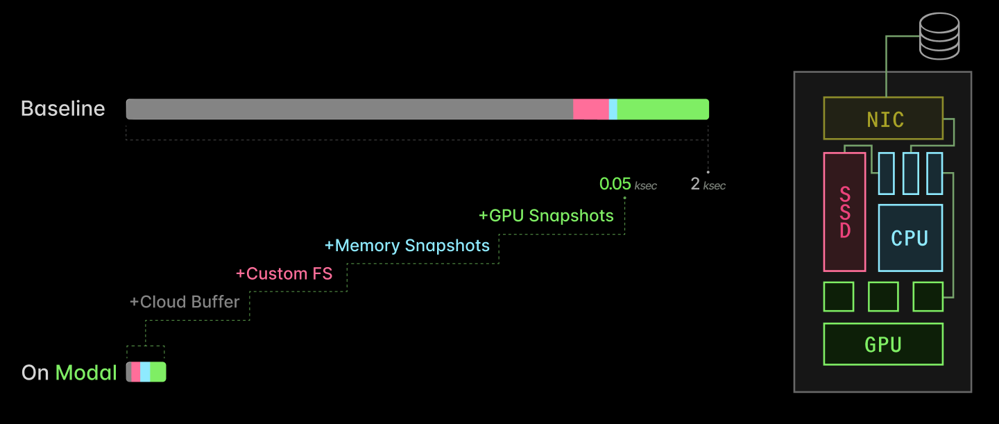
Modal は、推論ワークロードの予測不可能性に対応するため、サーバーレス GPU のスケーリング時間を数キログ秒から数十秒に短縮する技術的突破を達成した。
キーポイント
推論とトレーニングのスケーリング特性の違い
トレーニングは予測可能で定型的なワークロードである一方、推論(Inference)は変動が激しく不確実性が高いため、サーバーレスアーキテクチャとの親和性が極めて高い。
スケーリング速度の劇的な改善
従来のアプローチでは数キログ秒(数千秒)かかっていた新しいレプリカの起動時間を、Modal の技術により数十秒レベルまで短縮することに成功した。
真のサーバーレス GPU 実現への道筋
需要変動に即座に対応できる高速なリソースプロビジョニングが可能になることで、コスト効率とパフォーマンスを両立する「真の」サーバーレス GPU 環境が構築可能となる。
影響分析・編集コメントを表示
影響分析
この記事は、AI インフラストラクチャの根本的な課題である「推論ワークロードの変動性に対するリソース応答速度」を解決する具体的な技術的進歩を示しています。これにより、企業はオンデマンドで高コストな GPU リソースを維持することなく、変動する需要に柔軟かつ経済的に対応できるようになります。
編集コメント
推論コストの最適化において、スケーリング速度が鍵となることを示唆する重要な記事です。特に変動の激しい実サービス環境での運用効率化に直結する知見と言えます。
私たちは推論の時代にあります。数十億から数兆パラメータを持つニューラルネットワークが、毎秒数京回の演算を行う専用アクセラレータ上で実行され、大規模な メディア生成、ソフトウェアの作成、そして タンパク質の折りたたみ を行っています。
推論ワークロードは、以前を支配していたトレーニングワークロードよりも変動が大きく予測が困難です。そのため、アプリケーションを(仮想)マシンの上位レベルで定義し、変動する負荷に応じてより容易にスケールアップ・ダウンできるようにする*サーバーレスコンピューティング*にとって、自然な適性があります。
しかし、サーバーレスコンピューティングが機能するのは、新しいレプリカが需要の変化に合わせて迅速に起動できる場合に限られます。その変化は数秒単位で起こることもあります。例えば、B200 上で数十億パラメータの LLM を処理する SGLang の新しいインスタンスを素朴な方法で起動しようとすると、数十分かかったり、GPU の可用性のために何時間も停止したりすることがあります。
Modal では、この問題を解決するために過去 5 年間にわたって深いエンジニアリング作業を行ってきました。この記事では、その取り組みについて詳しく解説します。
重要な要素は 4 つあります:
- クラウドバッファ:新しい負荷を引き受けるために、健全でアイドル状態の GPU を少数量保持する
- カスタムファイルシステム:コンテンツアドレス型かつ多層構成のクラウドネイティブキャッシュから、コンテナイメージを遅延ロードして提供
- チェックポイント/復元:プロセスを直接メモリに復元することで、CPU 側の初期化処理をスキップ(高速化)
- CUDA チェックポイント/復元:CUDA コンテキストを直接メモリに復元することで、GPU 側の初期化処理をスキップ(高速化)
これらにより、AI 推論サーバーのレプリカスケールが数キログ秒から数十秒へと劇的に短縮されます。
私たちはこれまで、この取り組みの一部を ビット や ピース として共有してきました。なぜなら、秘密主義は優れた参入障壁ではないと考えているからです。また、より多くの人々が GPU を効率的に使いこなせるようになれば、市場で利用可能な GPU の数も増えるはずです。
しかし、今回のブログ記事では、初めてこの物語の全体像を一つの場所にまとめました。私たちのシステムが 購入する価値 があること、あるいはそれを構築するために 私たちに参加すること の意義があることを、ぜひご理解いただければ幸いです。
なぜサーバーレス GPU にこだわるのか?推論ワークロードにおける GPU アロケーション利用率の最大化のため
まず、問題を明確に定義しましょう。GPU は高価かつ希少であるため、その 利用率 を最大化する必要があります。ここでいう「利用率」とは、以下の無次元量を指します:
Utilization := Output achieved ÷ Capacity paid for
利用効率とは、達成された出力を支払い容量で割ったものです。利用効率を測定する方法は多数あり、出力と容量の定義も様々です。ここで最も洗練され、かつ厳格な指標はおそらく「モデル FLOP/s 利用率(Model FLOP/s Utilization)」であり、これは純粋なアルゴリズム演算要件を集積演算帯域幅で割ることで算出されます。
これはエンジニアにとって格好の話題です。また、「ヒーローラン」と呼ばれる大規模トレーニングにおいて特に重要であるため、多くの投資と注目を集めています。例えば最近では、誰もが xAI の約 10% の MFU を批判したという話題も取り上げられました。
しかし、スタックの另一端には、推論ワークロードにおいて達成された出力と割り当てられた容量との関係を崩壊させる、より基本的な利用効率の形態が存在します。それが GPU *アロケーション*利用率(GPU Allocation Utilization)です:
GPU Allocation Utilization := GPU-seconds running application code ÷ GPU-seconds paid for
「GPU 利用率」用語に関する補足 nvidia-smi や同様のツールが報告する「GPU 利用率」とは、この二つの極端な指標の中間に位置します。これは GPU 上で実行されている*カーネルコード*の時間の割合を報告するものであり、文字通り GPU 上で CUDA ストリームが動作している時間の割合を示しています。
詳しくはこちらをご覧ください
こちら。
推論アプリケーションは規模において非常に可変性があります。トレーニングとは異なり、容量に対する需要はエンジニアリング組織による直接的な制御や管理の外にあります。むしろ、これは外部のユーザー行動、すなわち市場やソーシャルメディアのアルゴリズム、あるいは製品チームによって駆動されます。
推論アプリケーションをモデル化するために使用する時間変化するポアソン過程からの 1 分あたりのリクエスト数のサンプルトレースを示します。季節変動(日次サイクル)だけでなく、平均需要が増加するにつれて需要の変動性が長期的に増大している傾向にも注目してください。
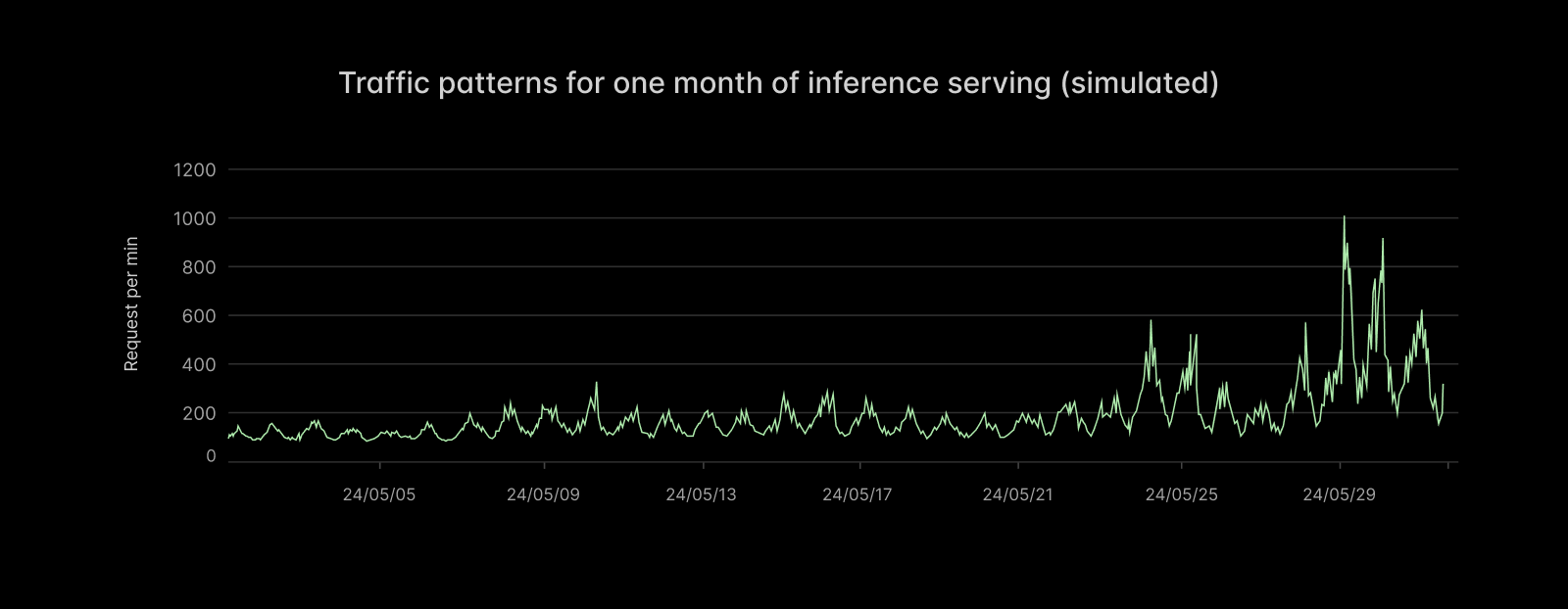
スパイク状の需要は深刻なエンジニアリング上の課題を提起します。AWS の Marc Brooker 氏から借用すれば:「システムの費用は(短期的な)ピークトラフィックに比例して増大しますが、ほとんどのアプリケーションにおいてシステムが生成する価値は(長期的な)平均トラフィックに比例して増大します。」スパイク状の需要とは高いピーク対平均比を意味し、これはシステム経済性に挑戦をもたらします。
具体的に想像してみましょう。このようなアプリケーションのための容量計画について。遅延目標内でリクエストを処理するために必要な GPU 数で測定される需要が以下のようなものであると仮定します:
固定された過剰な GPU 割り当てでは、利用率は低くなる
- 2月17日 午前06時、午前09時、正午、午後03時、午後06時、午後09時、午後10時、GPU 100枚。予測される負荷を適切に処理するために、140枚の GPU を割り当てます(ラックへの設置やハイパースケーラーでのレンタル)。しかし、それらの GPU の多くは時間の大部分がアイドル状態です——GPU アロケーション利用率は低くなります。私たちは自分の利益のために話しているのだと非難されるかもしれません。しかし、私たちだけがそう指摘しているわけではありません!Hebbia 氏の優れたブログ記事も参照してください。そして、単なる感覚ではなくデータがあります:2024年の「スケールにおける AI インフラストラクチャの現状」レポートによると、ピーク需要時に稼働している組織の大半は、70% 未満の GPU アロケーション利用率しか達成できていません。実際の GPU アロケーション利用率は、一般的に10〜20% に近いことがよくあります。固定割り当てでは、予期せぬスパイク発生時に需要が供給を上回ることがあります。それらを予測しようとするとコストがさらに増大し、収益の増加以上にコストが増えることになります。
サーバーレス GPU が難しい理由:起動レイテンシ
即効性のある解決策は、オートスケーリング容量のプロビジョニングです:需要が増加すれば供給も増やす。これを素朴に行うと、実際には問題が悪化します。
アロケーションが遅ければ、利用率と QoS(サービス品質)が損なわれる
2月17日 午前06時、午前09時、正午、午後03時、午後06時、午後09時、午後10時、GPU 100枚。最適化を行わない場合、ハイパースケーラーの API リクエストから実行中のサービスレプリカに至るまでに、数十分かかることもあります。以下の作業が必要です:新しいインスタンスを起動してヘルスチェックを行う(数分から数十分)、アプリケーションプログラムとファイルシステムの状態を読み込む(数分)、ホスト上でアプリケーションプログラムを開始し、リクエスト処理の準備を整える(数十秒)、デバイス上でアプリケーションプログラムを開始し、リクエスト処理の準備を整える(数分から数十分)。この間中、負荷は容量を超え、QoS は通常低下します(より高い並行度やキューに吸収され、結果として尾部レイテンシが膨らむか、最悪の場合は 503 エラーが発生する)。つまり、怒ったユーザーが生じます。もし容量のオンライン化に時間がかかりすぎると、一時的なスパイクを見逃すことさえあります。しかし、需要の不確実性とアロケーションの難しさを考慮すると、その容量は通常、長く低利用率のまま残ることになります。
Modal では、GPU 上での推論アプリケーションの起動時間を、従来の数十分から数秒から数十秒にまで最適化しました。これらの最適化により、多様な GPU 推論アプリケーションが「真にサーバーレス」で実行可能となりました。つまり、システム需要に対して供給をきっちりマッチングさせたプロビジョニングが可能になるのです。
高速な自動割り当てにより、利用率と QoS の両方を高く保つことが可能に
- 2月17日午前3時、午前6時、午前9時、正午、午後3時、午後6時、午後9時、午後10時、GPU。このドキュメントの後半では、クラウドストレージシステムやマシン管理からローカルディスク、CPU、そしてもちろん GPU に至るまで、上記の4つのステップ全体にわたって私たちが採用したエンジニアリングアプローチと実装したパフォーマンス最適化について説明します。これらの最適化を組み合わせることで、Modal 上での推論が40倍高速になり、起動時間が2千秒から50秒に短縮されます。推論サーバーは、素直な起動では2千秒以上かかるものですが、Modal では約50秒で起動します。この速度向上を実現する主要なアーキテクチャ最適化は、それらが対象とする主要システムコンポーネント(GPU と GPU メモリ、CPU と CPU メモリ、ローカルソリッドステートディスク(SSD)、またはマシン/インスタンス管理)によって色分けされ、示されています。本稿全体でこの配色と図解を使用します。
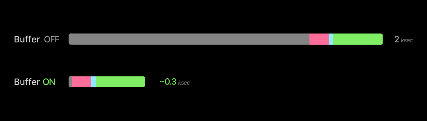
インスタンスの割り当てとヘルスチェックをホットパスから外すことで、数十分の遅延を削減できます。
レプリカの起動における最初のステップを考えてみましょう:新しいインスタンスを起動し、そのヘルスチェックを行う(数分から数十分かかります)。これを事前に行うことで、ホットパスから除外できます。具体的には、多くのアプリケーションで共有されるアイドル状態で健全な GPU のバッファを事前に用意しておき、新しいレプリカをこれらのユニットにスケジューリングし、非同期で新しいデバイスをバッファ内に起動します。また、レプリカがシャットダウンする際にバッファが大きくなりすぎた場合は、ユニットの割り当てを解除することも可能です。このバッファの管理は、他の場所で記述したように、面白い線形計画法の問題です。
割り当てられたマシン上に、すぐに使用可能だが未使用の機械を少量バッファリングしておくことで、新しいレプリカを空のマシン(明るい色で示されている)に迅速にスケジューリングできます。バッファからのリクエスト処理により、レプリカの起動にかかる遅延が数十分短縮されます。
システムレベルおよびアプリケーションレベルのバッファに関する補足 単一のワークロードを実行している場合(マルチワークロードシステムではない場合)、なぜインスタンス割り当てだけを「ホットパス」から外してバッファに移すのか、と疑問に思うかもしれません。セットアップ作業のより多くをバッファに移せないのでしょうか?もちろん可能です!Modal ユーザーは、リクエストに応答する準備ができているレプリカでアプリケーション層のバッファを維持できます buffer_containers。しかしそれでも、特定の規模のスpike を吸収するために必要なバッファのサイズは、新しいレプリカを作成できる速度に依存して拡大するため、以下の最適化は単一ワークロードシステムにおいても依然として重要です。
バッファを実行することは、ピーク時の割り当て利用率を 100% 未満に制限します。これは妥当なトレードオフです。なぜなら、100% の利用率は一般的に幻像だからです。CPU や IOPS(入出力オペレーション数)などの他のリソースの利用率が高くなりすぎた際に、新しいレプリカを起動したり、エンジニアにページを送ったりするのが一般的な慣行であることを考慮してください!
これは堅牢性にとって重要です。100% 稼働しているシステムにはエラーの余地がなく、そのため障害は日常的に故障へと直結してしまいます。私たちは個人的に、生活にもっとバッファ(余裕)を持たせることをお勧めします。例えば、洗面所に予備の歯ブラシを一つ用意しておくこと、重要なデバイスの充電器を自宅、オフィス、そして持ち歩く際にそれぞれ持っておくことです。
このバッファは、単一のシステム上でより多様なワークロードを受け入れる際にも特に有用です。Modal では、本番環境でのサービス提供だけでなく、「開発」ワークロードの多様化も積極的に支援しています。なぜなら、新しい開発環境を迅速に作成できるからです。追加のメリットとして、これらの環境はデフォルトで再現可能であり、本番運用可能なインフラ上で動作します。本番環境とのギャップを埋めることは、開発速度の向上にも寄与します。
肝心なのは、もちろん詳細です。重要なポイントの一つは、GPU にはヘルスチェックが不可欠だということです。GPU は他のハードウェア、特に回転ディスクのような notoriously(悪名高い)に繊細なコンポーネントと比較しても、はるかに高い確率で故障します。私たちは GPU のヘルスチェックシステムについて詳しくこちらで解説しています。要約すると、私たちの経験では、起動時に短いアクティブなヘルスチェックを実行し、その後に発生する可能性のある健康上の問題を監視する必要があります。ただし、より集中的なチェック(dcgmi diag など)は、より低い頻度(当社では週次など)に延期することが可能です。
- 月 03 水 05 金 07 11 月 09 火 11 木 13
0.05 0.10 0.15 0.200 Xid エラー/時間/GPU
GPU あたり 1 時間あたりの Xid エラー数(匿名化されたクラウドごとにグループ化)。故障率は無視できるレベルではありません!
コンテナの起動時間を数分から数秒に短縮するには、コンテンツアドレス型キャッシュからファイルを遅延ロードして提供する必要があります。
さて、次のステップを考えましょう:アプリケーションプログラムとファイルシステムの状態を読み込む(数分)
現在の慣行では、これは通常 1 つ以上のコンテナまたは仮想マシンを起動することを意味します。
おおよそ、コンテナとは、限られた権限を持つプロセスを支えるルートファイルシステムです。多数のコンテナを分散配置する場合、パフォーマンスはワーカーインスタンス上でのルートファイルシステムの構築がボトルネックとなります。
OS ディストリビューションのルートファイルシステムは非常に重く、ファイル数は数万に及び、サイズもギガバイト単位になります。素朴な方法では、docker run などのコマンドでその全体を読み込む必要があり、通常クラウド Ethernet がサポートする数 GB/秒の速度で行われます。さらに悪いことに、コンテナイメージは複数のレイヤーに分かれており、これらは順次適用されなければなりません。
解決策は、コンテナ*ランチャー*(Docker なら runc、gVisor なら runsc)とコンテナ*イメージ配信*を分離することです。私たちは libfuse を用いて構築した独自ファイルシステム「ImageFS」を使用しており、これは遅延ロードとマルチティア型のコンテンツアドレス型キャッシュを組み合わせたもので、クラウドプロバイダの特性に最適化されるように設計されています。
カスタムファイルシステムで実装しているコンテナの高速起動のための鍵となる「トリック」は、賢明に(すべての優れたエンジニアがそうするように)遅延ロードすることです。コンテナイメージには、世界中の時刻情報やロケール情報など、多くのアプリケーションが決して読み込まないファイルが含まれています。コンテナ起動前にファイルシステム全体を読み込むのをスキップし、代わりにメタデータ(インデックス)の読み込み開始時にブロックするだけで済みます。メタデータは数メガバイト程度なので、コンテナを起動するために必要な他のすべての要素とともに、100 ミリ秒以内で読み込むことができます。
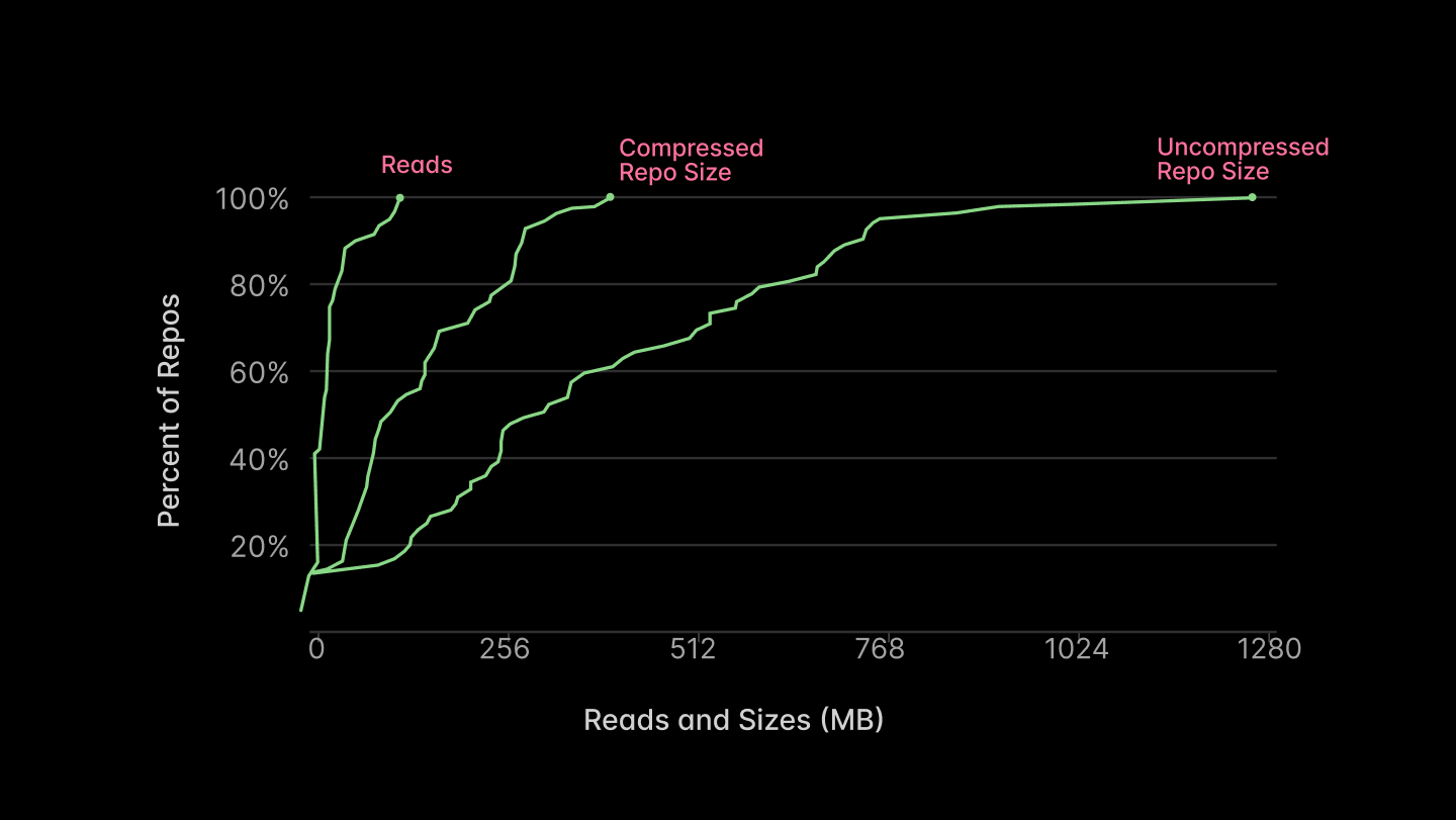
残りのファイルは、他の処理と並行してロードするか、あるいは全くロードする必要もありません。図 5 に示されている USENIX FAST '16 の Slacker paper の報告によると、ファイルの大部分は読み込まれません(以下に再掲)。
現在、このファイルシステムは libfuse を用いて実装されています。これはユーザー空間で Linux ファイルシステムを記述するためのライブラリです。カーネルは、標準的なシステムコールを使用してファイルを操作する 1 つのユーザー空間プログラムと、新しいファイルシステムを実装するもう 1 つのプログラム(最終的には独自のシステムコールを持ち、そのうちの 1 つがカーネルを経由して元のプログラムに返ってくる)の間を仲介します。これは、カーネルモジュール内にカスタムファイルシステムを実装する場合よりも、構築や配布がはるかに簡単です。
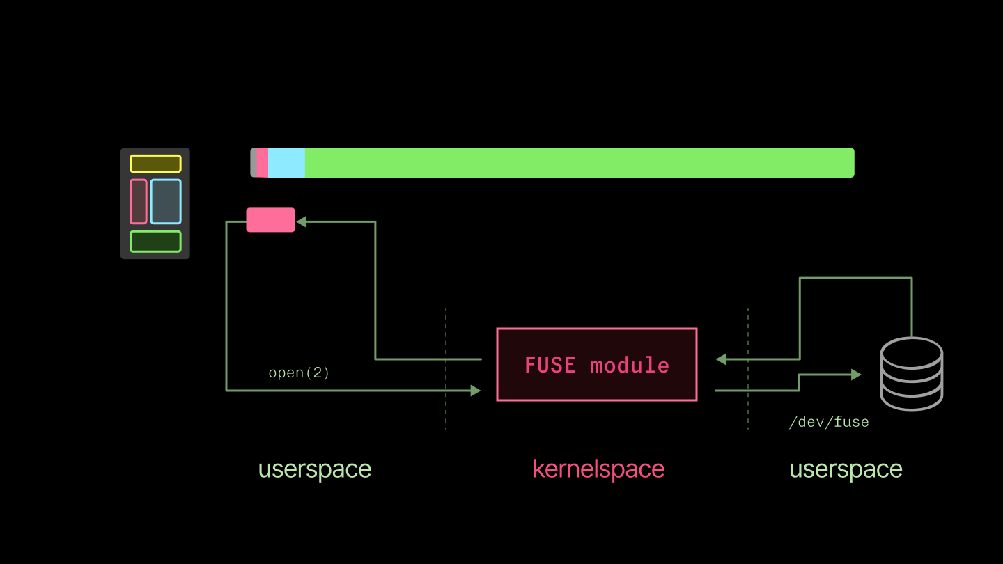
代償として、ユーザー空間とカーネル空間の間でコンテキストスイッチが倍増します。これはターミナル文字デバイスの読み出しなど、レイテンシが支配的なワークロードでは痛みを伴うものですが、私たちが利用するスループットが支配的なワークロードへの影響は小さくなります。パフォーマンスへの影響に関する有用な詳細分析については、To FUSE or Not to FUSE from USENIX FAST '17 をご覧ください。
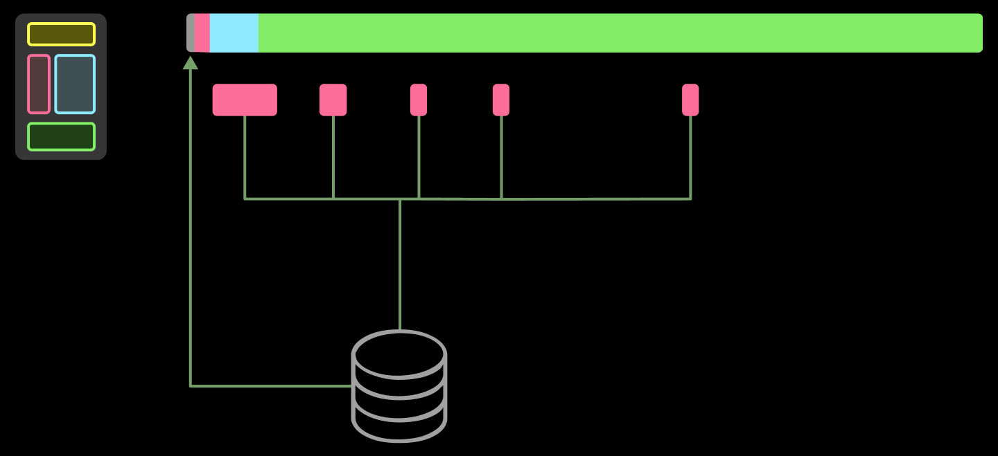
しかし、無料の昼食はありません:コンテナによって実際にアクセスされるすべてのデータは依然として読み込まれる必要があります。もし典型的なコンテナがアクセスする数千ものファイルをオブジェクトストレージから無謀にも一つずつ取得しようとすれば、「コンテナ起動」から torch.cuda.is_available まで到達するのに数時間かかってしまいます。そこで、もう一つの重要な構成要素となるのが、我々が積極的に(ただし非同期で)充填する階層化されたコンテンツアドレス型キャッシュです。
コンテナ間でのイメージ内容の重複が極めて大きいため、私たちは*コンテンツアドレス型*キャッシュを採用しています。多くの推論アプリケーションは同じソフトウェア(例:Python, PyTorch, CUDA stack)を使用します。
しかし、パスベースのキャッシングや Docker のレイヤーごとのキャッシングでは性能を十分に引き出せていません。例えば、共有されるバイト列が必ずしも同じコンテナイメージの層に存在するとは限りません。
 image
image
キャッシュは、クラウドプロバイダーが提供するストレージの階層構造に対応させるために、CPU や GPU 内部のキャッシュと同様に*ティアリング(多段化)*されています。以下の図と表には、主要なコンポーネントとそのスループット、レイテンシ、コストが記載されています。
システム | 読み込みレイテンシ (μs) | 読み込みスループット (GiB/s)
---|---|---
ページキャッシュ (Page Cache) | 0.001 - 0.1 | 10-40
SSD | 100 | 4
AZ キャッシュサーバー (AZ Cache Server) | 1,000 | 10
リージョン CDN | 100,000 | 3-10
Blob ストレージ | 200,000 | 3-10
主要な転換点は以下の通りです:
- メモリ:Linux のページキャッシュ。これが主たるメモリ内ターゲットです。マイクロ秒単位のレイテンシを実現できる唯一の選択肢であり、高いスループットを誇りますが、容量は限られています(RAM は高価であり、さらに価格が高騰しています)。
- ディスク:ローカルのソリッドステートドライブ (SSD)。SSD は回転ディスクに比べてメモリからの段差がはるかに緩やかですが、依然として体感できるレベルです。私たちは大容量のドライブを用意し、最も頻繁に使用されるコンテンツで急速に埋め尽くします。
- ネットワーク経由:Blob/オブジェクトストレージ。これは実質的に無限の容量を持ち、ハイパースケーラーが保存するデータを格納するための資金を尽きる前に、ユーザー側がデータ転送のコストで資金を尽きてしまいます。ただし、レイテンシは非常に高くなります。このレイテンシによるペナルティは厳しいものですが、多くのクラウド構成ではピーク帯域幅がディスクよりも高い場合がある点に注意してください。
これを本当に機能させるためには、SSD とオブジェクトストレージの間にさらに層を追加することも検討できます。例えば、RDMA レイヤーや同一 AZ 内でのピアツーピア共有などです。どちらも数値上は魅力的ですが、エンジニアリングの複雑さが大幅に増すため、現時点では導入していません — まだです。
合計して、コンテナの起動時間を 1 分短縮できました。起動に数秒しかかからない単純なアプリケーションにとっては、これは絶対的なゲームチェンジャーです。LLM 推論サーバーのような重いアプリケーションにおいては、数分かかる起動時間から約 1 分を削減できます。
速度向上の決定的な要因をもたらす大きなアーキテクチャ上の動きに続き、今度は数パーセントポイントの微調整という地道な作業が続きます。この微調整の詳細についてはこちらのブログ記事で解説しました。以下にいくつかのハイライトを挙げます。
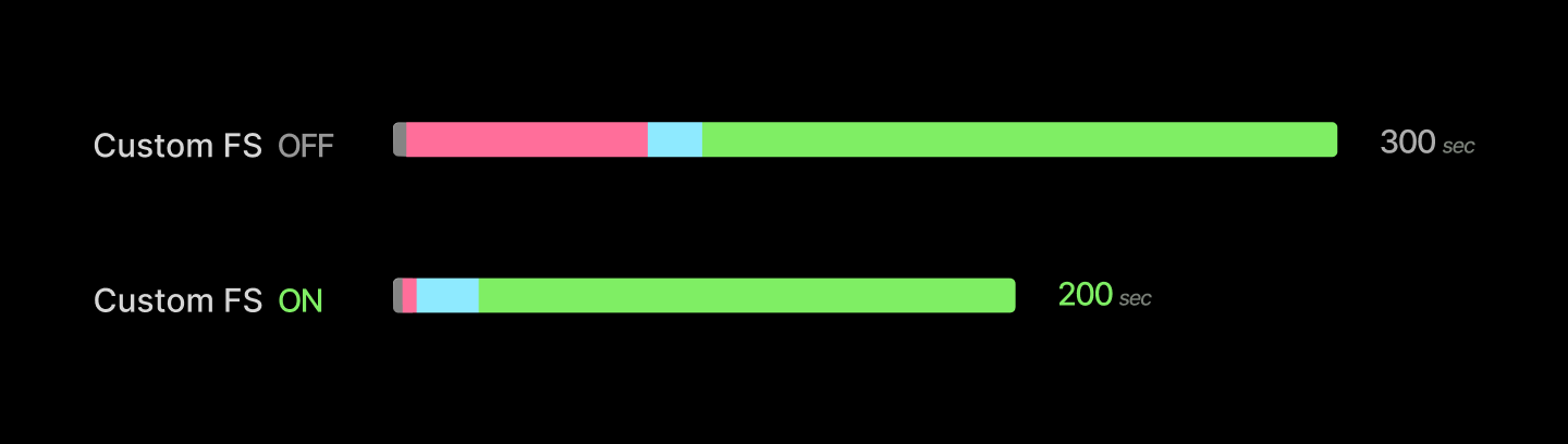
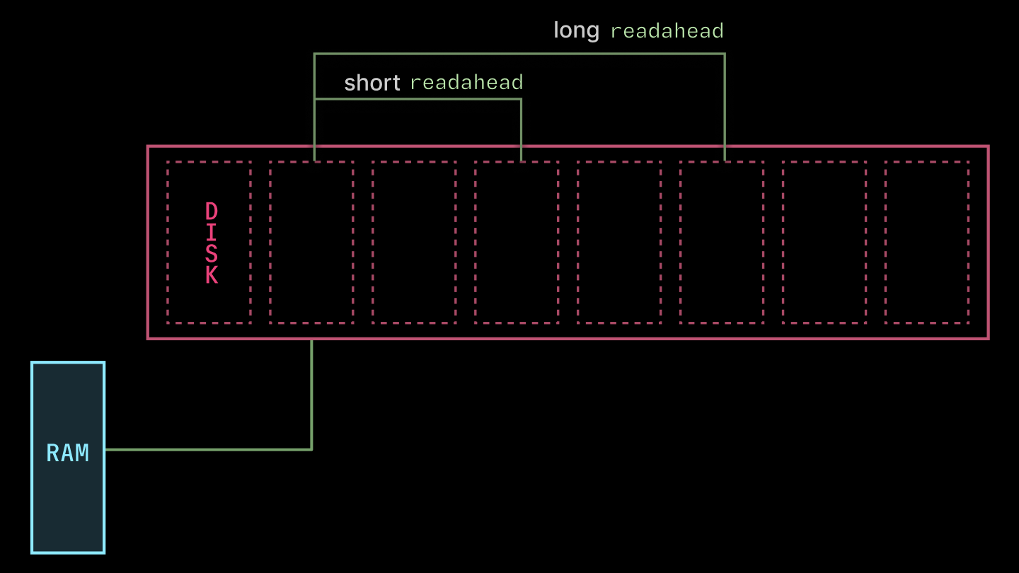
まず、libfuse にはパフォーマンスに関するいくつかの設定項目(ノブ)が用意されています。私たちは、各リクエストに対してカーネルが事前に読み込むキロバイト数を指示する read_ahead_kb を調整することで最も大きな効果を得ました(下図参照)。この値をデフォルトの 128 から 32 * 1024 に引き上げました。コンテナイメージの読み込みには大量の読み取り処理が必要となるため、より大きな値が有効です。あまりにも高い値(ギガバイト単位)にすると、深刻なスラッシングが発生しました。
第二に、コンテナイメージレイヤーの gzip 非圧縮・圧縮処理をスキップします。DEFLATE は本質的にシングルスレッド(LZ77, Huffman)であり、スループットが約 100 MB/s に制限され、これはキャッシュ層のいずれのスループットよりもはるかに低くなります。コンテナイメージ作成に完全な制御権がある場合は、転送中の帯域幅を節約し、非圧縮時のネットワークボトルネックを回避するために zstd を使用し、画像圧縮における初期コストを負担することを選択できるかもしれません。しかし、私たちはまた、特に 動的エージェントワークロードのより良いサポート のために、イメージ作成を高速に保つよう努めています。
CPU メモリスナップショットにより、アプリケーションホスト側の起動にかかる数十秒をスキップできます。
さて、3 つ目のステップについて考えましょう:
- ホスト上でアプリケーションプログラムを開始し、リクエスト処理の準備を整える(数十秒)
これは、アプリケーションのコンテナプロセスが開始された時点から、最初の「有用な」作業である最初のリクエストの処理が始まる時点に至るまでに必要なすべての作業を包含します。
例えば、Python 文 import torch を実行することを考えてみましょう。これにより、数千行に及ぶ Python コードが起動され、その中にはさまざまなファイルの読み込みやドライバとの対話を目的とした数万回のシステムコールの実行が含まれます。典型的な推論アプリケーションで使用されるすべてのライブラリに対してこれを繰り返すと、「プロセス開始」と「リクエスト実行中」の間には多くの秒数分の作業が必要になります。
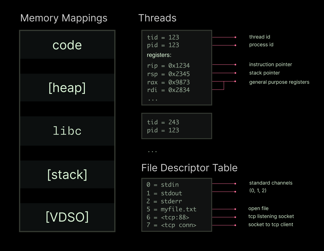
ここで重要な洞察は、実行中のプロセスとはヒープ、いくつかのスレッド、およびファイル記述子テーブルの集合体であるということです。このような構造になります:
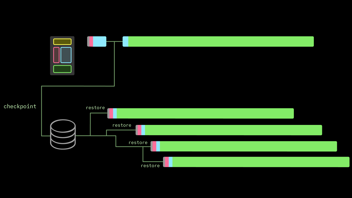
この状態を再現できれば(「チェックポイントを作成する」)、実行中のプロセスも再現できます(「チェックポイントから復元する」)。その状態を適切にパッケージ化すれば、ストレージからプロセスを再構築する方が、新規コピーを実行して再構築するよりも高速になります。
これが、トランスペアレントなチェックポイント/復元インターフェースの核心となる考え方です。*トランスペアレント(透過的)*である理由は、ユーザープログラムがチェックポイント作成や復元が行われていることを意識する必要がないからです。Linux におけるトランスペアレントなチェックポイント/復元の実装は、Checkpoint/Restore In Userspace (CRIU) と呼ばれます。透過的な C/R は、実行中のプログラムを異なるマシンへ移行するなどの用途に有用です。しかし、私たちの主要目標がコールドスタート時間の短縮であるため、トランスペアレントなチェックポイント/復元は当システムにおける必須要件ではありません。
そのため、私たちはコンテナライフサイクル管理インターフェースを通じてユーザーに C/R インターフェースを公開しています。その様子は以下のようになります:
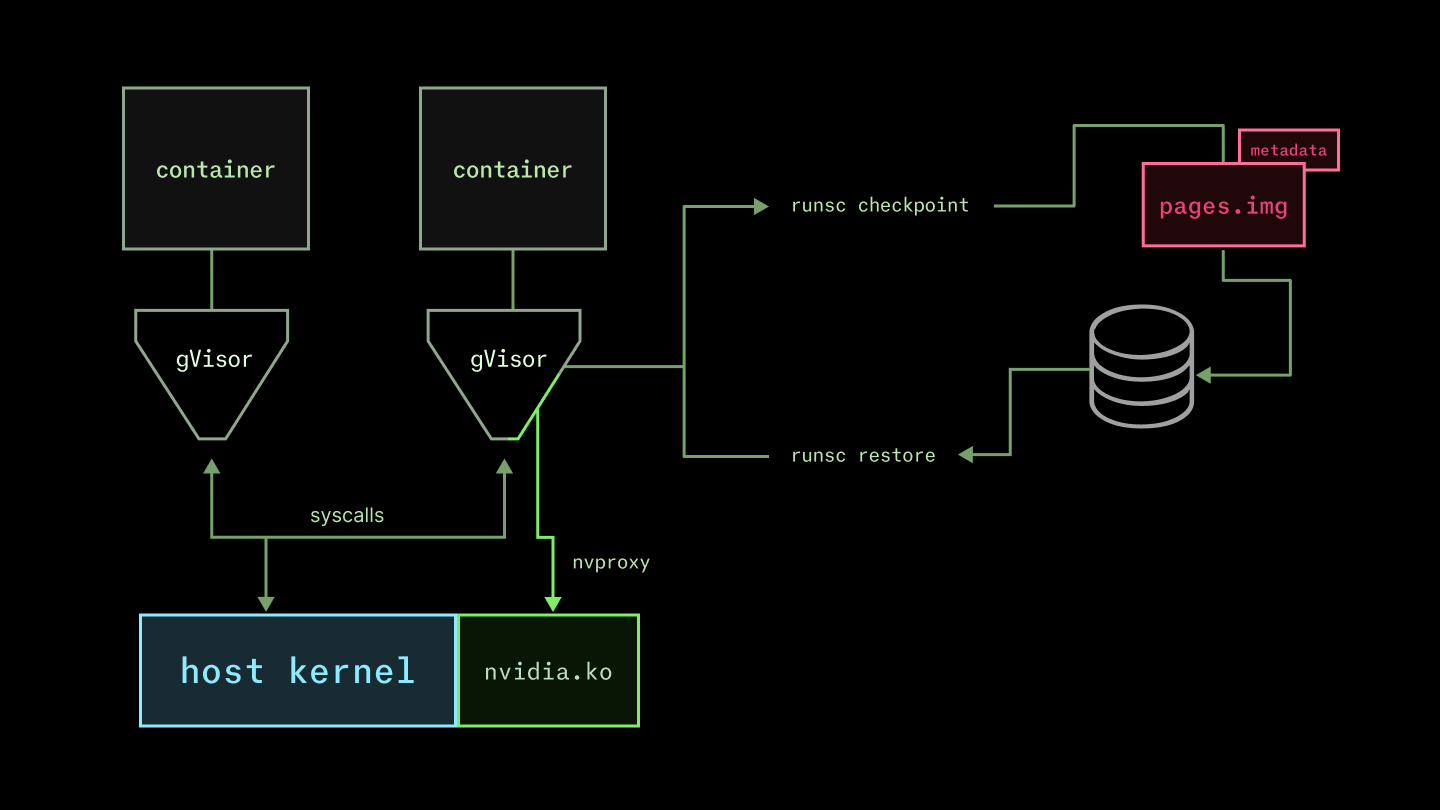
現在、Linux のチェックポイント/リストア(C/R)は使用していません。ユーザーコンテナには gVisor の runsc を実行しており、これはユーザースペース内で Linux カーネルの一部を効果的にエミュレートします。この限定的な表面領域により、最近特定された CVE-2026-31431、別名「CopyFail」 などの脆弱性攻撃から自動的に保護されます。私たちは特に nvproxy サブコンポーネントに関心があり(貢献もしています!)、これは GPU の カーネルモードドライバ と通信します。
アプリケーションはこのエミュレートされたカーネルとのみインターフェースするため、ホストカーネルの協力を得ることなく、チェックポイントおよびリストアが可能になります。runsc におけるチェックポイント/リストアは実際には非常に容易です。runc ランタイム内のコンテナは単純に状態機械(state machine)として機能します。つまり、ランタイムは Go で実装されており、非同期/待機(async/await)スタイルの並行処理を持つ他のシステムと同様に、協調的プリエンプションを持つタスクのコレクションとして設計されています。システムはすでに各待機ポイントで中断され、その後継続されているため、「単に」その状態をシリアライズしてチェックポイント化するだけの問題です。
より正確には、runsc の checkpoint コマンドはコンテナを停止し、disk 上に状態を生成します。これにより、runsc restore を使用してコンテナを再起動することが可能になります(詳細はこちら:docs here)。デフォルトでは圧縮されたアーカイブ形式ですが、私たちは圧縮なしで生成しています(gzip のボトルネックを思い出してください!)。重要なファイルは pages.img で、これは生のページデータを含んでいます。サイズは少なくとも 100 MB ですが、多くの GB に達することもあり得ます(ただし、一般的にシステムメモリを超えることはありません)。
他にも多くの要素が関わっていますが、チェックポイントの復元性能は、これをホスト側のページキャッシュにどれだけ速く読み込めるかにかかって決まります。私たちは上記で説明したカスタムファイルシステム機構を使用して、チェックポイントファイルを配信しています。
その結果、新しいレプリカのホスト側コンポーネントを読み込むまでの時間が約 10 分の 1 に短縮されました。当社のメモリスナップショットシステムについては、こちらのブログ記事 で詳しく読むことができます。
import torch
1s<li
原文を表示
We are in the age of inference. Billion- to trillion-parameter neural networks are run on specialized accelerators at quadrillions of operations per second to generate media, author software, and fold proteins at massive scale.
Inference workloads are more variable and less predictable than the training workloads that previously dominated. That makes them a natural fit for *serverless computing*, where applications are defined at a level above the (virtual) machine so that they can be more readily scaled up and down to handle variable load.
But serverless computing only works if new replicas can be spun up quickly — as fast as demand changes, which can be at the scale of seconds. Naïvely spinning up a new instance of, say, SGLang serving a billion-parameter LLM on a B200 can take tens of minutes or stall for hours on GPU availability.
At Modal, we’ve done deep engineering work over the last five years to solve this problem. In this blog post, we walk through what we did.
There are four key ingredients:
- Cloud buffers: maintain a small buffer of healthy, idle GPUs to take on new load
- Custom filesystem: serve container images lazily out of a content-addressed, multi-tier cloud-native cache
- Checkpoint/restore: fast-forward through CPU-side initialization by directly restoring processes into memory
- CUDA checkpoint/restore: fast-forward through GPU-side initialization by directly restoring CUDA contexts into memory
Together, they take AI inference server replica scaling from multiple kiloseconds to just tens of seconds.
We’ve shared bits and pieces of this work along the way, because we believe that secrecy is a bad moat. And if more people learn how to use GPUs efficiently, there will be more available in the market for us!
But this blog post represents the first time we’ve put the entire story together in one place. We hope it convinces you that our system is worth buying into — or joining us to build it.
Why care about serverless GPUs? To maximize GPU Allocation Utilization for inference workloads.
First, let’s frame the problem clearly. GPUs are expensive and scarce, so we want to maximize their utilization, where “utilization” is the following unitless quantity:
Utilization := Output achieved ÷ Capacity paid for
There are many ways to measure utilization — to define output and capacity. The most sophisticated and most stringent here is probably “Model FLOP/s Utilization”, which divides raw algorithmic operation requirements by aggregate arithmetic bandwidth.
This is catnip for engineers. It’s also especially critical for “hero run” large-scale training, so it draws a lot of investment and attention, e.g. recently as everyone dunked on xAI’s ~10% MFU.
But at the other end of the stack, there’s a more basic form of utilization that wrecks the relationship between achieved output and allocated capacity for inference workloads, GPU *Allocation* Utilization:
GPU Allocation Utilization := GPU-seconds running application code ÷ GPU-seconds paid for
Aside on "GPU Utilization" terminology The "GPU utilization" reported by nvidia-smi and similar tools is in between these two extremes. It reports the fraction of the time that *kernel code* is running on the GPU — literally, the fraction of time there is a CUDA stream running on the GPU. Read more
here.
Inference applications have highly variable scale. Unlike training, the demand for capacity is outside the direct control and management of the engineering organization. Instead, it is driven by external user behavior — by markets or social media algorithms or product teams.
Here’s a sample trace of requests per minute from a time-varying Poisson process we use to model inference applications. Notice not only the seasonal variation (daily cycles) but also the long-term trend of increasing variability in demand as the average demand increases.
Spiky demand raises serious engineering problems. To borrow from Marc Brooker of AWS: “the cost of a system scales with its (short-term) peak traffic, but for most applications the value the system generates scales with the (long-term) average traffic.” Spiky demand means high peak-to-average ratios, which challenge system economics.
Concretely, imagine the capacity planning for such an application. You might have demand (measured in GPUs required to service requests within latency targets) that looks like this:
With a fixed, over-provisioned GPU allocation, utilization is low
- Feb 1703 AM06 AM09 AM12 PM03 PM06 PM09 PM100 GPUs To properly service your anticipated load, you allocate (rack-and-stack, rent on a hyperscaler) 140 GPUs. But most of those GPUs sit idle most of the time — the GPU Allocation Utilization is low. You might accuse us of talking our book here. But we aren’t the only ones to call this out! See the excellent blog post by Hebbia. And we have data, not just vibes: according to the State of AI Infrastructure at Scale report in 2024, the majority of organizations achieve less than 70% GPU Allocation Utilization when running at peak demand. Actual GPU Allocation Utilizations are commonly often closer to 10-20%. With fixed allocations, demand can also exceed supply during unanticipated spikes. Trying to anticipate them just increases cost further — more than it increases revenue.
What’s so hard about serverless GPUs? Startup latency.
The immediate solution is to provision auto-scaling capacity: when demand increases, increase your supply. Done naïvely, this actually worsens the problem:
If allocation is slow, utilization and QoS suffer
Feb 1703 AM06 AM09 AM12 PM03 PM06 PM09 PM100 GPUs Without optimization, going from hyperscaler API request to a running service replica can take tens of minutes. You need to do the following: spin up a new instance and health-check it (minutes to tens of minutes)
- load application program and filesystem state (minutes)
- start the application program on the host, ready it to service requests (tens of seconds)
- start the application program on the device, ready it to service requests (minutes to tens of minutes)
During all of this time, load is in excess of capacity, and QoS typically degrades (absorbed into higher concurrency or queues and thus inflated tail latencies or, worse, 503s). That means angry users. If the capacity takes too long to come online, it can even miss a transient spike. But given the unpredictability of demand and the difficulty of allocation, that capacity typically sticks around, under-utilized, for an extended period.
At Modal, we’ve optimized the spin-up of inference applications on GPUs from many tens of minutes down to a few seconds or tens of seconds. With these optimizations, a wide variety of inference applications of GPUs can run “truly serverlessly”: with provisioned supply tightly matched to system demand.
With fast, automatic allocation, utilization and QoS can both be high
- Feb 1703 AM06 AM09 AM12 PM03 PM06 PM09 PM100 GPUs In the rest of this document, we will explain the engineering approach we took and the performance optimizations we implemented for each of the four steps above, which span the stack from cloud storage systems and machine management to local disks, CPUs, and, of course, GPUs. Together, these optimizations allow inference on Modal to spin up 40x faster: 50 seconds instead of 2k. Inference servers that take upwards of 2 kiloseconds to boot naïvely boot in ~50 seconds on Modal. The key architectural optimizations that achieve this speedup are indicated and color-coded by the key system component that they target -- GPUs and GPU RAM, CPUs and CPU RAM, local solid state disk (SSD), or machine/instance management. We use this color scheme and schematic throughout the post.
You can remove tens of minutes of latency by taking instance allocation and health checks out of the hot path.
Consider the first step in replica spin-up: spin up a new instance and health-check it (minutes to tens of minutes)
We can remove this from the hot path by doing it ahead of time: running a buffer of idle, healthy GPUs, shared by many applications, scheduling new replicas onto those units, and spinning up new devices into the buffer asynchronously. We can also de-allocate units when the buffer grows too large, as replicas spin down. Managing this buffer is a fun linear programming problem, as we’ve written elsewhere.
Servicing requests from the buffer removes tens of minutes of latency from replica spin-up.
Aside on system- and application-level buffers If you're running a single workload, rather than a multi-workload system, you might ask why we are only moving instance allocation out of the "hot path" and into the buffer. Can't we move more of our setup work into the buffer? And you can! Modal users can maintain an application layer buffer of replicas ready to service requests with
buffer_containers. But even then, the size of the buffer you need to absorb spikes of a given magnitude scales with the speed you can create new replicas, and so the optimizations described below are still important for single-workload systems.
Running a buffer limits the peak allocation utilization below 100%. This is a reasonable trade-off to make, since 100% utilization is generally a mirage. Consider that it is common practice to spin up new replicas and even page engineers when utilization of other resources, like CPU or IOPS, gets too high!
This is important for robustness. A 100% utilized system has no margin for error, and so faults routinely become failures. We can personally recommend adding more buffers to your life — keep an extra toothbrush in your bathroom; keep a charger for your critical devices at home, the office, and on your person.
This buffer is especially useful for accommodating a wider variety of workloads on a single system. At Modal, we’ve leaned into supporting a variety of “development” workloads, not just production serving, because we can quickly create a new development environment. As an extra win, these environments are reproducible-by-default and on prod-ready infra. Closing the gap with production infrastructure also improves development velocity.
The devil is, of course, in the details. One key piece: health checks are critical for GPUs, which fail at a much higher rate than other hardware, including notoriously finicky components like spinning disks. We wrote about our GPU health-checking system in detail here. The tl;dr is that, in our experience, you need to run a short active health check on boot and monitor for health issues that arise later, but you can defer more intense checks (like dcgmi diag) to a slower cadence (for us, weekly).
- Mon 03Wed 05Fri 07Nov 09Tue 11Thu 130.0500.1000.1500.200Xid errors / hr / GPU Critical level Xid errors per hour per GPU, grouped by (anonymized) cloud. Failure rates are far from negligible!
You can cut container start from minutes to seconds by serving files lazily out of a content-addressed cache.
Now let’s consider the next step: load application program and filesystem state (minutes)
In contemporary practice, this generally means booting up one or more containers or VMs.
Roughly, a container is a root filesystem backing a process with limited permissions. For distributed deployments of many containers, performance is bottlenecked by the construction of the root filesystem on the worker instance.
Root filesystems of operating system distros are thicc — tens of thousands of files, gigabytes in size. Naïvely, with a command like docker run, you need to load that whole thing, typically at the few GB/s supported by cloud Ethernet. Even worse, the container image is split into several layers, which must be applied sequentially.
The solution is to disaggregate the container *launcher* (runc for Docker, runsc for gVisor) from the container *image delivery*. We use a custom filesystem we call ImageFS, built with libfuse, that combines lazy loading with a multi-tiered, content-addressed cache designed to match cloud provider affordances.
The key “trick” for fast container start that we implement in our custom filesystem is to be lazy, judiciously (as all good engineers do). Container images contain many files, like timezone and locale information for the entire world, that will never be read by most applications. You can skip loading the entire filesystem before the container starts and instead just block start on loading metadata (an index). The metadata is only a few megabytes, so it can be loaded in 100ms or less, along with everything else needed to start a container.
The remainder can be loaded concurrently with other work — or not at all! The majority of the files will not be read, as reported in Figure 5 of the Slacker paper from USENIX FAST ‘16, reproduced below.
We currently implement this filesystem with libfuse. It’s a library for writing Linux filesystems in userspace. The kernel intermediates between one userspace program using standard system calls on files and another implementing a new filesystem (with, in the end, its own syscalls, one of which eventually returns to the original program by way of the kernel). This is much simpler to build and distribute than a custom filesystem in a kernel module.
There’s a price: you have double the context switches between userspace and kernelspace. This can be painful for latency-dominated workloads, like reading from a terminal character device, but has less of an impact on throughput-dominated workloads, where we use it. For a useful detailed breakdown of the performance implications, see To FUSE or Not to FUSE from USENIX FAST ‘17.
But there’s no free lunch: all the data that *is* accessed by the container still needs to be loaded. If you naïvely fetched each of the thousands of files accessed by a typical container from object storage, getting from “container start” to torch.cuda.is_available would take hours. So the other key component is a tiered, content-addressed cache that we fill eagerly (but asynchronously).
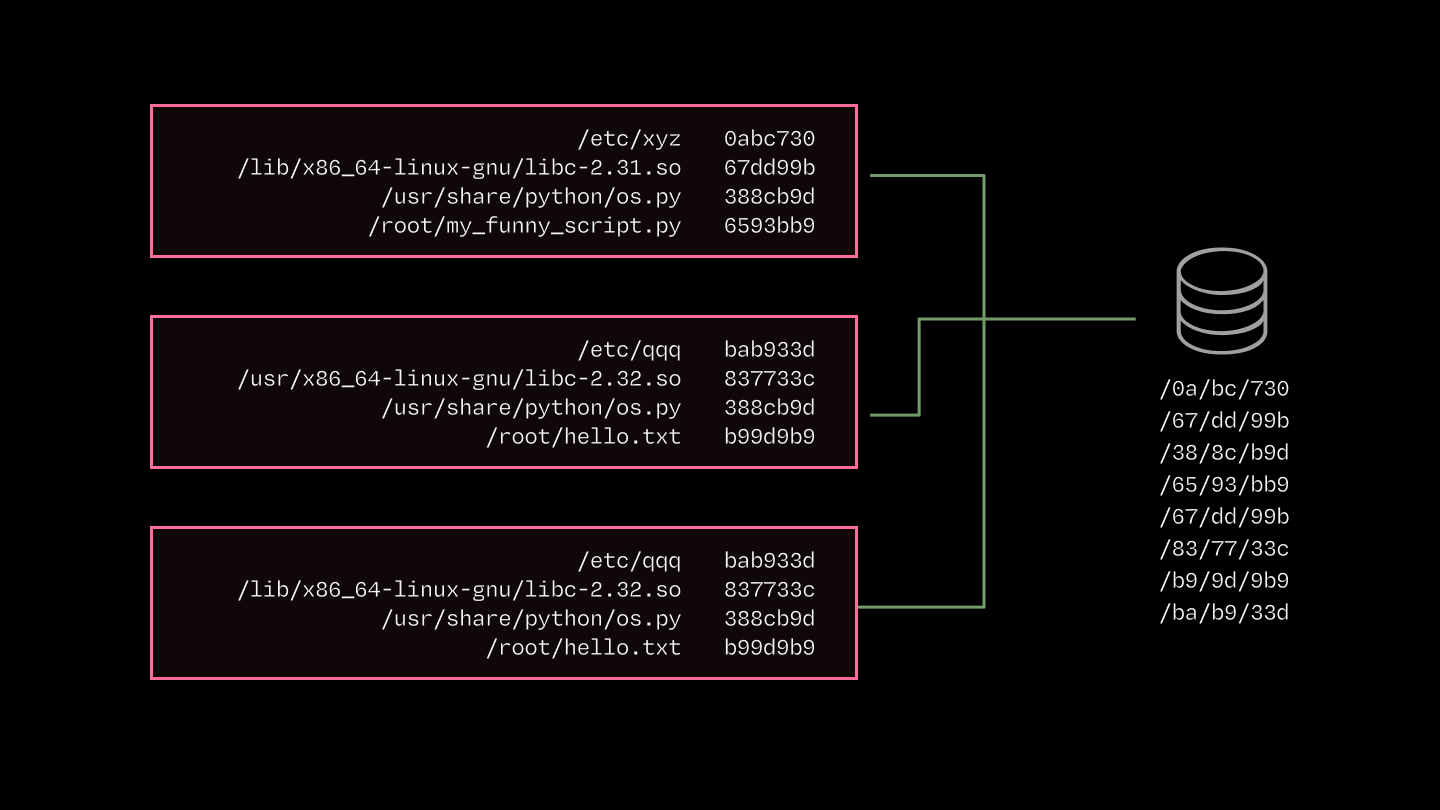
We use a *content-addressed* cache because the overlap in image contents across containers is huge. Many inference applications use the same software (e.g. Python, PyTorch, CUDA stack).
But path-based cacheing and Docker’s layerwise cacheing leave performance on the table. For instance, shared bytes aren’t guaranteed to be in the exact same container image layer.
The cache is *tiered*, just like the caches inside CPUs and GPUs, to map onto the hierarchy of storage available on cloud providers. The diagram and table below list the key components and their throughputs, latencies, & costs.
SystemRead Latency (us)Read Throughput (GiB/s)
Page Cache0.001 - 0.110-40
SSD1004
AZ Cache Server100010
Regional CDN100,0003-10
Blob Storage200,0003-10
The key breakpoints are:
- Memory: Linux page cache. This is the primary in-memory target. It's your only option for microsecond latencies and has high throughput, but capacity is limited (RAM is expensive, and getting dearer).
- Disk: Local solid state. SSDs are a much gentler step down from memory than spinning disks, but still noticeable. We grab big drives and rapidly fill them up with the most commonly-used content.
- Over-the-network: Blob/object storage. This has essentially infinite capacity — you will run out of money pushing bytes before the hyperscalers run out of money storing them. But it has much higher latency. That latency penalty is punishing, but note that the peak bandwidth can be higher than disk in many cloud configurations!
To really make this rip, you might build more layers between SSD and object storage, like an RDMA layer or within-AZ peer-to-peer sharing. Both are compelling on the numbers, but add a lot of engineering complexity, so we haven’t added them — yet.
Altogether, we’ve cut container start times down by a minute. For simple applications whose spin-up takes only a few seconds, this is an absolute gamechanger. For heavier applications like an LLM inference server, it removes about a minute from a several-minute start.
The big architectural moves that give integral factors of speedup are followed by a grind of percentage points. We detailed that grind in this blogpost. Here’s a few highlights.
First, libfuse exposes some knobs for performance. We found the most juice from tuning the read_ahead_kb, which directs the kernel to read that many kilobytes ahead of each request (as depicted below). We increased the value from the default 128 to 32 * 1024. The bigger value is nice for the large-read-heaviness of container image loading. Much higher values (in the gigabytes) caused gnarly thrashing.
Second, we skip gzip de/compression of container image layers. DEFLATE is inherently single-threaded (LZ77, Huffman), which limits you to ~100 MB/s, much lower than the throughput of any of the cache layers. If you have full control over container image creation, you might choose to use zstd and pay an upfront cost in image compression to save bandwidth during transfer and avoid bottlenecking the network during decompression. But we also try to keep image creation fast, especially to better support dynamic agent workloads.
You can fast-forward through tens of seconds of application host-side startup with CPU memory snapshotting.
Now, let’s consider our third step:
- start the application program on the host, ready it to service requests (tens of seconds)
This encompasses all of the work that needs to be done to go from the point where the application’s container process is started to the point where the first “useful” work is started — processing the first request.
Consider, for instance, executing the Python statement import torch. This kicks off thousands of lines of Python code that, among other things, executes tens of thousands of syscalls to load a variety of files and interact with drivers. Repeat that for all of the libraries used in a typical inference application, and you’ve got many seconds of work to do between “process start” and “request in-flight”.
The key insight here is that any running process is a heap, some threads, and a file descriptor table. Something like this:
If you can recreate that state (”create a checkpoint”), you can recreate the running process (”restore from checkpoint”). Package that state right, and you can recreate a process from storage faster than you can recreate it by executing a fresh copy.
That’s the core idea behind transparent checkpoint/restore interfaces — *transparent* because user programs do not need to be aware that they are being checkpointed and restored. The implementation of transparent checkpoint/restore in Linux is called Checkpoint/Restore In Userspace (CRIU). Transparent C/R is useful for, among other things, migration of live programs onto different machines. Because our primary goal is to reduce cold start time, transparent checkpoint/restore is not a requirement in our system.
So we expose the C/R interface to users via our container lifecycle management interface. It looks something like this:
We don’t use Linux C/R currently. We run user containers with gVisor’s runsc, which effectively emulates (a subset of) the Linux kernel in userspace. This limited surface area provides automatic protection from exploits like the recently-identified CVE-2026-31431, bka “CopyFail”. We’re particularly interested in (and contribute to!) the nvproxy sub-component, which communicates with the GPU’s kernel-mode drivers.
Because applications only interface with this emulated kernel, they can be checkpointed and restored by it without cooperation from the host kernel.
Checkpoint/restore is actually especially easy for runsc. A container in the runsc runtime is straightforwardly a state machine. That is, the runtime is architected (in Go) as a collection of tasks with cooperative preemption, as in most other systems with async/await-style concurrency. The system is already being interrupted and then continued at every await point, so it’s “only” a matter of serializing that state into a checkpoint.
More precisely, the runsc checkpoint command stops a container and produces state on disk that can be used to restart the container with runsc restore (docs here). By default, it’s a zipped archive, but we generate without compression (remember the gzip bottleneck!). The key file is pages.img, which contains the raw page data. It is at least 100 MB but can be many GB (though generally not larger than system memory).
There’s a lot of other moving pieces, but checkpoint restoration performance is won and lost on how quickly this can be brought into the host page cache. We use the same custom filesystem machinery described above to deliver the checkpoint files.
The result is about a 10x reduction in time to load the host-side components of a new replica. You can read more about our memory snapshotting system in this blog post.
import torch
1s<li
関連記事
今日のまとめ
AI日報で今日の重要ニュースをまとめ読み