Sonar Vortex、AI コーディングエージェントの CI チェックパターンを革新
本文の状態
日本語全文を表示中
詳細モードで約22分の本文を読めます。
同じ出来事の情報源
この情報源を基点に整理
TLDR AI
TLDR AI は、カスタマイズ性を重視した新しい米国製AIモデルの設計思想について解説する記事を発表したが、具体的な企業名や技術詳細は本文に明記されていない。
AI深層分析を開く2026年8月20日 22:04
AI深層分析
キーポイント
記事の主題と形式
TLDR AI が公開した本記事は、「カスタマイズ可能に設計された新しい米国製AIモデル」を主題としており、読了に約26分を要する長文分析となっている。
設計思想の焦点
記事は既存の汎用モデルとは異なり、ユーザーや組織が自らのニーズに合わせて柔軟に調整・カスタマイズできることを主眼としたモデル設計を論じている。
情報の限界性
提供されたテキスト断片には画像の埋め込みコードが含まれるのみであり、具体的な開発企業名や技術仕様に関する記述は含まれていないため、詳細な分析は不可能である。
Inkling モデルのアーキテクチャ的特徴
66層で各層に256のエクスパートを持ち、トークンごとに6つだけ活性化されるMixture-of-Experts構造を採用している。
Thinking Machines のミッションと製品戦略
同社はAIが人間の意志と判断を拡張することを使命とし、既存のファインチューニングサービス「Tinker」に続き、Scratchから訓練された初のモデル「Inkling」を発表した。
重要な引用
The New American AI Model Designed to be Customized
(26 minute read)
Thinking Machines, founded by Mira Murati (the ex-CTO of OpenAI), describes its mission as building AI that extends human will and judgment.
Inkling is the company's first model trained from scratch.
編集コメントを表示
編集コメント
提供されたテキスト断片には具体的な企業名や技術詳細が含まれていないため、分析の深さは限定的となる。記事タイトルが示す通り「カスタマイズ性」に焦点を当てた内容であると推測されるが、実態を確認するには完全な本文が必要である。
Source Article
元記事を日本語で読む
本文に関係しない購読案内、埋め込み通知、サイト内プロモーションは除いています。
AI コーディングエージェントはコードを素早く生成できますが、CI チェックは通常、エージェントの作業完了後に実施されます。Sonar Vortex はこのパターンを変えます。Sonar Vortex はエージェントのコーディングループ内で動作し、記述前にアーキテクチャの文脈を提供するとともに、生成する過程でリアルタイムに出力を検証します。内部テストでは、トークン消費量が 36% 減少し、欠陥が 92% 減ることが確認されました。
Thinking Machines は 2026 年 7 月 15 日、「Inkling」というモデルを発表しました。その導入部でいくつか興味深い点が指摘されています。
- Inkling は 66 層から構成され、各層には 256 のエキスパートが格納されていますが、任意のトークンに対して活性化するのはそのうち 6 つのみです [2]。
- ほとんどの層は直近の短いテキストウィンドウしかアクセスできませんが、一部の層では全テキストにアクセス可能です [1]。
- 単語の位置情報は、多くの研究機関が数年前から採用しなくなった手法でエンコードされています。
ミラ・ムラティ(OpenAI 元 CTO)が設立した「Thinking Machines」は、そのミッションを「人間の意志と判断を拡張する AI の構築」と定義しています。同社は主に 4 つの方向性で活動しており、強力なモデルの訓練、ユーザー自身の知識でモデルをカスタマイズできるツールの開発、人間と機械間のコミュニケーションチャネルを広げるインターフェースの構築、そしてモデルがどのように作られるかに関する研究論文の発表です [3]。
「Inkling」以前に同社は、「Tinker」というオープンモデルのファインチューニングサービスを提供していましたが、Inkling は同社がゼロから訓練した最初のモデルとなります [1]。重みは Apache 2.0 ライセンスの下で Hugging Face に公開されており [2]、誰でもダウンロードして独自のデータで再訓練することが可能です。
本記事では、Thinking Machines が Inkling を構築する際に下したさまざまな選択について解説します。主なトピックは以下の通りです。
- エキスパートの混合(Mixture of Experts)と、9750 億パラメータから 410 億パラメータへの縮小におけるギャップ
- 100 万トークンのコンテキストウィンドウを支える、ローカルアテンション層とグローバルアテンション層の組み合わせ
- 位置エンコーディング:現在の標準手法ではなく、Thinking Machines が採用した旧来のアプローチ
- 画像や音声が入力される仕組み:事前に訓練されたエンコーダーを介さずに直接モデルへ取り込まれる方法
- 「思考の強さ(Thinking effort)」:0 から 1 の間で調整可能な設定値で、回答前にモデルがどの程度推論を行うかを制御します。
*免責事項:本記事は、各種ソースから公開された情報に基づいています。末尾に参考文献を記載しています。不備や誤りにお気づきの場合はコメントをお願いします。*
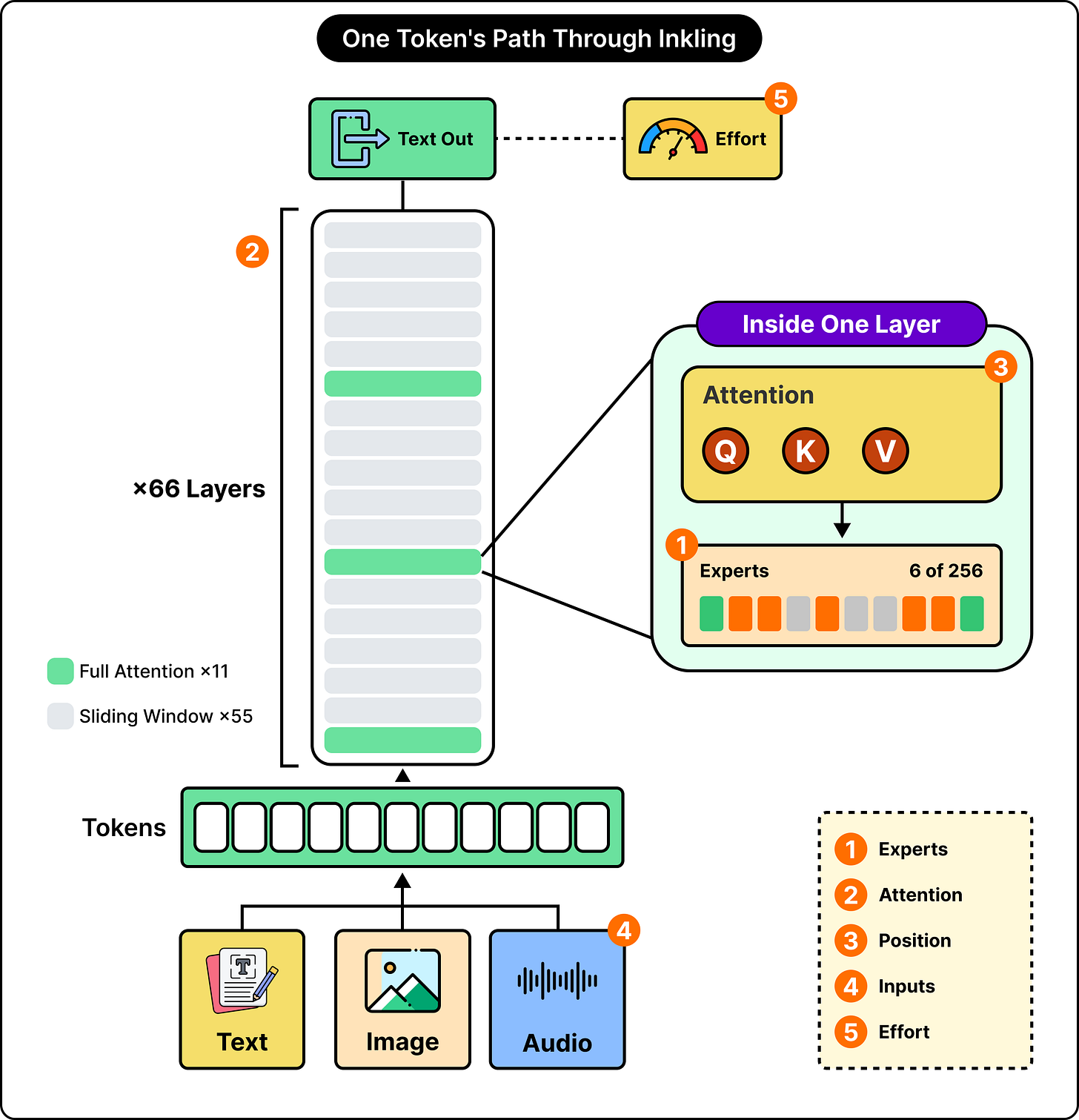
以下の図は、これら 5 つの要素がモデル内でどのように配置されているかを示しています。
まず、このアーキテクチャを理解するために重要な 4 つの用語を確認しておきましょう。
トークン:テキストの断片のことです。モデルは文よりも小さく、通常は単語よりも少し小さい単位で処理を行います。例えば、「Inkling was released in July」という一文は、6 つのトークンに分割されることがあります。一般的な単語は 1 トークンとして扱われますが、珍しい単語は 2〜3 トークンに分けられます。
パラメータ:モデル内部に保存されている一つの数値のことです。これは学習過程で獲得されたものです。「モデルには 9750 億個のパラメータがある」という表現は、ファイル内に格納されている個別の数値の総数を指します。これらはすべてランダムなノイズから始まり、モデルが意味のあるテキストを生成するまで数百万回にわたって調整されます。
トレーニング:モデルにテキストを見せさせ、次のトークンを予測させることで機能します。その予測結果と実際に出現したトークンを比較し、より良い予測になる方向へパラメータをわずかに調整します。この調整の大きさや方向は「勾配」と呼ばれ、これらを一括で計算する手順は「逆伝播(backpropagation)」と呼ばれます。これを数兆回のトークンにわたって繰り返すことで、パラメータは有用な予測を生み出す値へと収束していきます。
レイヤー:トークンが処理される過程における1つの段階です。Inkling には、順序立てて積み重ねられた 66 個のレイヤーが存在します [2]。トークンの表現はレイヤー 1 から入り、変換を経てレイヤー 2 へ、そして最終的にレイヤー 66 まで通過し、そこで次のトークンを予測します。各レイヤーには、同じく 2 つの部分があります。
一つは、シーケンス内の他のトークンから情報を引き出すアテンションステップです。
もう一つは、その結果を変換するフィードフォワードステップです。
Inkling は、モデルを保存するためのコストと実行するためのコストを分離しています。これが、これほど大規模なモデルでも利用可能な価格で提供できる理由です。
通常のトランスフォーマーでは、各レイヤーのフィードフォワードステップは単一のネットワークであり、すべてのトークンがその全体を通り抜けます。もしそのネットワークに 50 億個のパラメータが含まれている場合、処理されるすべてのトークンに対して、その 50 億個すべてが関与することになります。
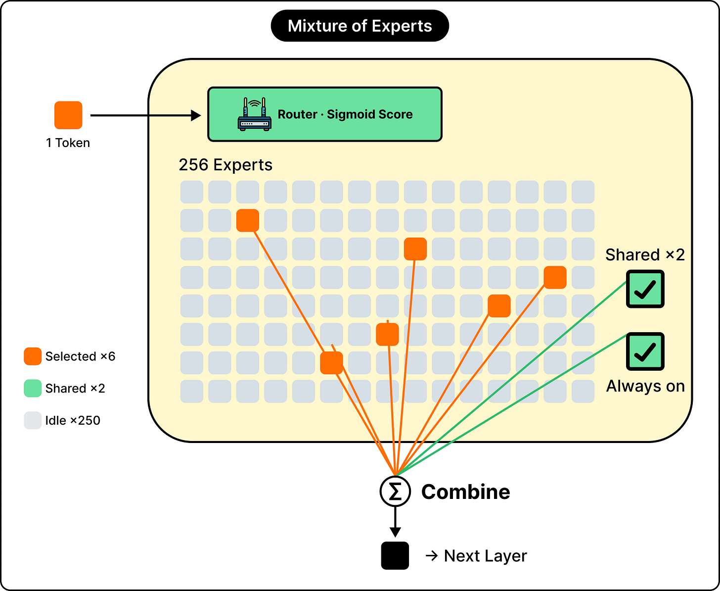
Inkling はこの単一ネットワークを置き換え、256 個の小さなネットワーク、つまり「エキスパート」を用意しています。各トークンに対しては、選択ステップによって 256 個の中から 6 つが選ばれます。実際に実行されるのはその 6 つだけで、残りの 250 個はそのトークンについてはアイドル状態となり、代わりに他のトークンの処理を担当します [2]。この設計パターンは「エキスパートの混合(Mixture of Experts)」と呼ばれ、Thinking Machines は自社のバージョンが DeepSeek が発表したアプローチを主に踏襲していると述べています [1][8]。
以下の図をご覧ください:
簡単な例を通じて、この仕組みを理解してみましょう:
例えば、10 億パラメータを持つエキスパートを 10 個持つレイヤーを構築し、トークンごとにそのうち 2 つを使用する場合を考えましょう。
ディスク上のファイルには全 100 億のパラメータが含まれていますが、モデルを実行するにはそれらすべてをメモリに読み込む必要があります。単一のトークンを処理する際にも 20 億パラメータが必要となるため、同じ総規模の通常のレイヤーと比較すると、コストは約 5 分の 1 で済みます。
Inkling はこの仕組みを大規模に実装しています。モデル全体のパラメータ数は合計 9750 億ですが、単一のトークンを処理する際に実際に使用されるパラメータ数は約 410 億です [1]。これは、同時に稼働しているモデル全体の約 4% に相当します。
ハードウェア要件を考えると、この仕組みの効率がより明確になります。チェックポイントとは、学習済みの全パラメータを保存したファイルのことです。Inkling のフル精度(full-precision)チェックポイントには、少なくとも 2TB の GPU メモリが必要です。モデルカードによると、これは NVIDIA B300 カード 8 枚、あるいは H200 カード 16 枚に相当します [2]。
Thinking Machines はまた、量子化(quantised)されたチェックポイントについても言及しています。これは、数値の精度を少し下げてパラメータを保存する方式です。例えば、3.14159265 を 3.14 と書くことでスペースを節約するのと同じ原理で、わずかな精度の低下と引き換えにデータサイズを削減します。この量子化バージョンでは約 600GB で済み、B300 カード 4 枚に収まります [2]。
漠然とした「フォワード・デプロイメントエンジニア(FDE)」の求人に対して、優秀な候補者は懐疑的です。タイトルだけで信頼を得ることはできません。
『2026年版 FDE 採用動向レポート』は無料で公開されており、候補者が何を求めているか、市場がどのように進化しているか、そして企業がこれらの役割をいかにわかりやすく説明すべきかが解説されています。
採用を検討中の方へ。ご自身の求人枠を、FDE に特化したジョブボード「forwarddeployedengineer.com」に掲載することも可能です。
256 人中から 6 名の専門家を選抜する作業は、一見簡単そうに見えますが、実際には決して単純ではありません。選考プロセスの詳細は以下の通りです。
「ルーター」と呼ばれる小さなコンポーネントが、すべてのエキスパートに対してスコアを生成します。
各エキスパートには、学習過程で獲得した独自の数値リストが付随しています。ルーターはこのリストと入力されたトークンの表現を比較し、両者の一致度が高いほど大きな数値(生スコア)を出力します。
この生スコアの値は任意の大きさになり得るため、シグモイド関数を通す必要があります。シグモイドは、あらゆる数値を入力として受け取り、0 から 1 の間の値に変換する数学的な関数です。例えば、8 を入力すると約 0.9997 が返され、0 を入力するとちょうど 0.5 になります。また、-4 を入力すると約 0.018 が得られます。非常に大きな正の数は 1 に近づき、非常に小さな負の数は 0 に近づきます。それ以外の値は、その中間のどこかに収束します。Inkling のルーターも、エキスパートのスコアを生成するためにこのシグモイド関数を利用しています [1]。
スコアリングが完了した後、上位 6 つのエキスパートが動作し、それぞれの出力が上記のスコアを重みとして用いて統合されます。スコアが 0.9 のエキスパートは、0.4 のエキスパートよりも結果に対してより大きな寄与を果たします。
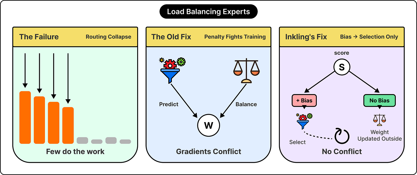
このアプローチには、特定の種類の失敗が発生する確率が高まるという欠点があります。その失敗を理解するには、数百万回の学習ステップにわたって何が起きるかを考える必要があります。例えば、たまたま初期段階で「エキスパート 47」が平均よりもわずかに多く選択されたと仮定しましょう。すると、より多くのトークンを処理することになり、それに応じて勾配更新の回数も増えます。その結果、隣接する他のエキスパートよりも急速に性能が向上します。性能が高まったことでルーターからのスコアも上がり、さらに多く選択されるという悪循環(あるいは好循環)が生じます。
このループを十分に長く実行すると、256 個のエキスパートを持つ層のうち、約 20 個がほぼすべての処理を担当し、残りの 236 個は未発達なままになる可能性があります。これを「ルーティング崩壊」と呼びます。つまり、256 個のエキスパートを保存するためにコストを支払ったにもかかわらず、実際には 20 個分の機能しか得られないのです。
これにはもう一つの課題もあります。エキスパートは通常異なるマシンに分散されているため、人気のある 4 つのエキスパートを保持するマシンがボトルネックとなり、その周辺のマシンが遊んでしまう状態が発生します [9]。
この問題に対する従来の解決策は、トレーニング目的関数にペナルティを追加する方法です。これはエキスパートの使用状況が偏った場合に大きくなるペナルティであり、モデルに対して同時に二つのことを学習させることになります。一つ目はトークンの予測を正しく行うこと、二つ目はエキスパートの使用バランスを保つことです。
しかし、この二つの目標は互いに逆方向に勾配を生成するという問題があります。予測の勾配が「このパラメータを増やせ」と指示する一方で、バランス維持のためのペナルティは「減らせ」と指示します。どちらかが勝ってしまいますが、いずれにせよモデルは本来目指すべき方向から引き離されてしまいます。もしペナルティの強度を高く設定すればテキスト品質が低下し、逆に低く設定すればエキスパートは結局崩壊してしまいます [9]。
Thinking Machines は、Wang らによって導入され、DeepSeek にも採用された手法を使用しています [1][8][9]。この方法は、各エキスパートごとに独立したバイアス値を保持することで、この対立構造そのものを解消します。これは単に各エキスパートのスコアに追加される小さな数値です。肝心なのは、このバイアスをどこで適用するかという点にあります。
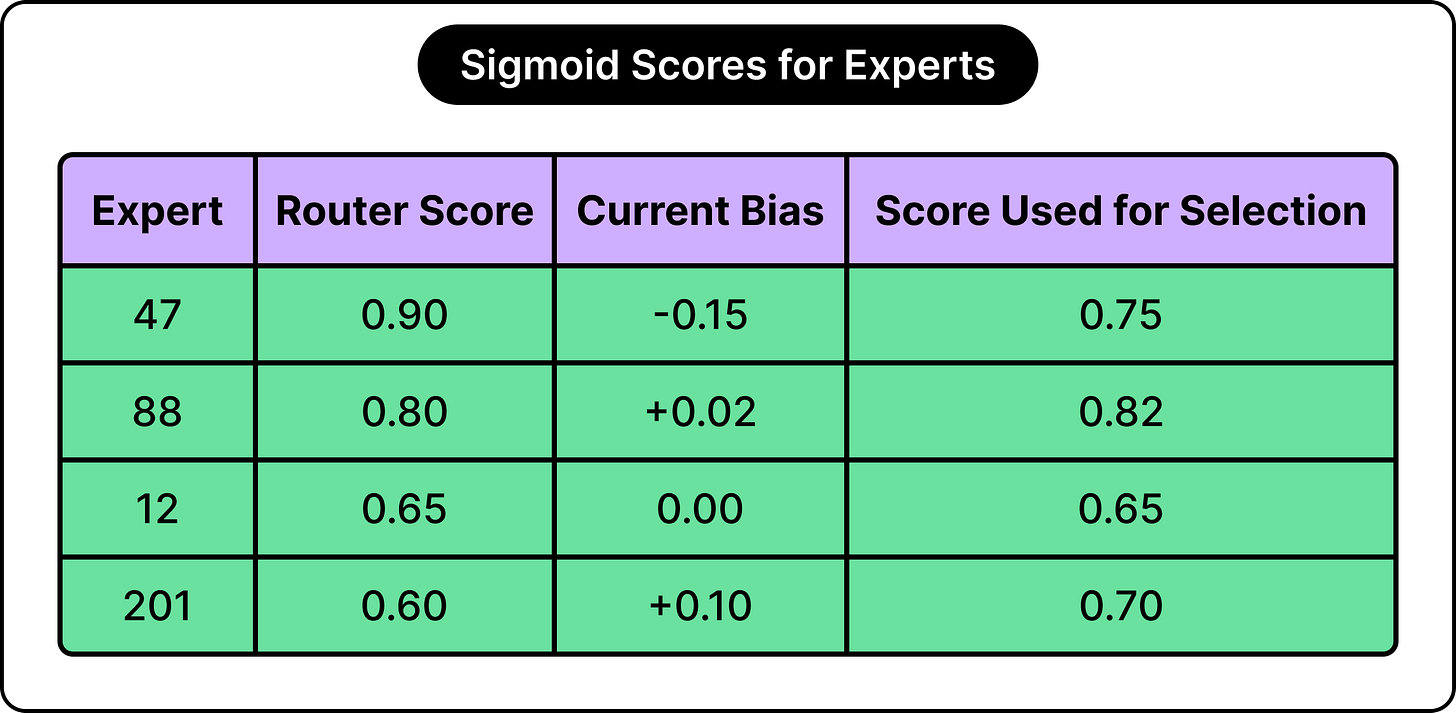
この構成において、トークンが層に到達する様子を順を追って見てみましょう。ルーターが 4 つのエキスパートに対して出力したシグモイドスコアを例に考えます。
エキスパート 47 は最近過負荷状態が続いているため、バイアスが -0.15 まで低下しました。これにより選択スコアがエキスパート 88 を下回り、代わりにエキスパート 88 がそのスロットを獲得します。このようにバイアスは、どのエキスパートが選ばれるかを左右する要因となります。
ただし、エキスパート 88 の出力が最終結果に組み込まれる際、重み付けは 0.80(元のルータースコア)で行われ、バイアスは適用されません。つまり、バイアスの影響は選択プロセスのみであり、重み付けには一切関与しません。また、このバイアス更新はバックプロパゲーションの外部で動作する単純なカウントルールによって行われます。
主な目的は、混雑したエキスパートの選定を抑制しつつ、比較的閑散としたエキスパートにも機会を与えることです。
その結果、専門的な利用がバランスよく保たれ、学習目標に対して競合する勾配は一切発生しません。
ここで注意すべき点は、ルーティングに関わらず、すべてのトークンに対して 2 つの追加の専門家が動作するということです。これらは「共有専門家」と呼ばれ、ほぼすべてのトークンが必要とする汎用的な処理を担当します。Thinking Machines によると、選択された 6 つのルーティング専門家と 2 つの共有専門家のスコアは、重みとして使用される前に正規化されます [1]。つまり、8 つすべてが共通の範囲にスケーリングされ、それぞれが比例して貢献することになります。言い換えれば、トークンあたり合計 8 つの専門家が動作します。
スパース性(Sparsity)はフィードフォワードステップのコストを処理します。一方、アテンションステップには独立したコストがあり、これははるかに急速に増大します。Inkling は、層の大部分が非常に少ないデータのみを検査することで、このコストを管理しています。
モデルは、すべてのトークンに対して 3 つの数値セットを計算します。
- クエリ:その位置に必要な情報の種類を記述するもの。
- キー:その位置が提供する情報の種類を記述するもの。
- バリュー:その位置から次に渡される実際のコンテンツを含むもの。
各トークンのクエリは、それ以前のすべてのトークンのキーと比較されます。一致度が高いほどスコアが高くなり、そのスコアに応じて、どの程度の割合で以前に登場したトークンのバリューが現在の位置に取り込まれるかが決定されます。これが、文の中で「it」という単語が、それが指し示す名詞と結びつく仕組みです。
すべてのトークンがそれ以前のすべてのトークンと比較されるため、比較回数はシーケンス長の二乗に比例して増加します。例えば:
トークン数 1,000 で約 100 万回の比較が発生し、10,000 トークンでは約 1 億回、そして 100 万トークンになると約 1 兆回の比較が必要になります。
Inkling は 100 万トークンのコンテキストウィンドウをサポートしていますが [2]、66 レイヤー全体で層ごとに 1 兆回の比較を行うのは、現実的なハードウェアでは到底実現不可能です。
そこで登場するのがスライディングウィンドウ方式のレイヤーです。これは各トークンがそれ以前のすべてのデータではなく、直近の固定数トークンのみを参照する仕組みです。ウィンドウサイズを 1,000 に設定すれば、50 万番目のトークンは 499,000〜500,000 番目のトークンとのみ比較を行い、それ以上は行いません。これにより比較回数は 50 万回から 1,000 回に減り、シーケンス全体の計算量は二乗ではなく直線的に増加します。
すると当然、疑問が生じます。「すべてのレイヤーが狭いウィンドウしか見ないなら、長い文書の 1 ページ目の情報がどうやって 400 ページ目に届くのか?」という点です。
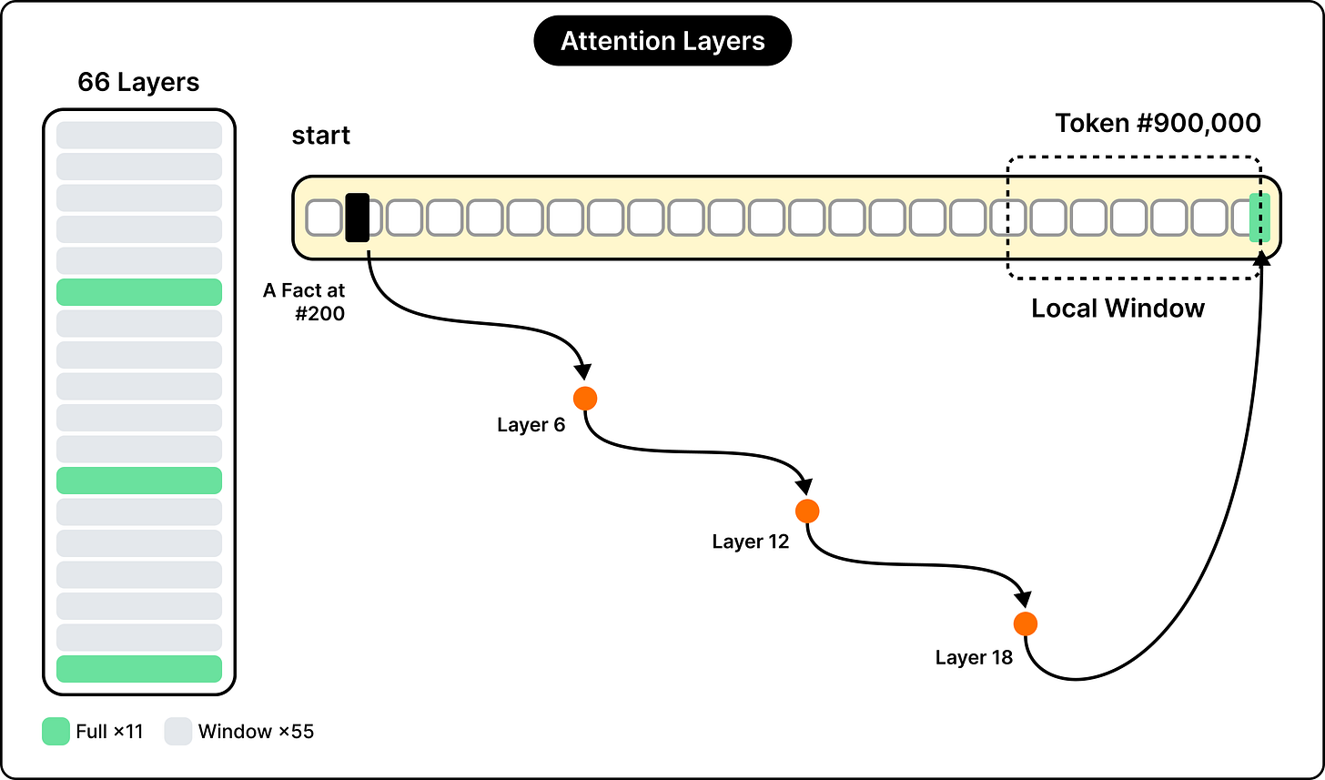
Inkling では、スライディングウィンドウレイヤーとフルアテンション(全結合)レイヤーを 5:1 の比率で交互に配置しています [1]。vLLM プロジェクトが公開した統合ノートでは、この 66 レイヤーの構成について具体的な数値が示されており、55 レイヤーがスライディングウィンドウ方式、残りの 11 レイヤーがフルアテンション方式であると明記されています [7]。
情報は、11 層のフルアテンション層を通過して伝播します。例えば、トークン 200 にある情報がトークン 900,000 の予測に重要である場合を考えましょう。6 番目の層(最初のフルアテンション層)では、位置 900,000 の表現が直接その情報を参照して取得できます。その後、この情報は局所的な表現の中で前方へ伝わり、12 番目の層で更新され、さらに 18 番目の層でも再度更新されます。このように、長距離の経路はおよそ 6 層に一度現れ、残りの 5 層では低コストで近傍の文脈を処理します。
Inkling はまた、8 つのキー・バリューヘッド [1] を採用しています。アテンション計算では通常、異なるクエリ、キー、バリューセットを用いて並列に複数回実行され、それぞれの並列コピーが「ヘッド」と呼ばれます。多くのクエリヘッドで少数のキーとバリューセットを共有することで、テキスト生成時に必要なメモリ量を削減しています。
この構成を簡略化して示した図は以下の通りです:
このアプローチには、一つの現実的な課題があります。長文脈モデルは大きなドキュメントの全体的な内容についてはよく処理できますが、その中間に埋もれた特定の詳細を見逃す可能性があります。
百万トークンを扱う場合、もう一つ問われるのは、モデルが各トークンがシーケンス上のどこに位置しているかをどのように表現するかという点です。
Thinking Machines は、現在の標準手法ではなく、古くからある技術を採用しました。その理由は、モデルが学習中に一度も経験したことのない長さのデータに対応するためです。
クエリとキーの比較には順序に関する情報が含まれていません。例えば、「猫が男を噛んだ」と「男が猫を噛んだ」はどちらも同じ 5 つのトークンで構成されています。位置情報を示すシグナルがない場合、アテンション処理では両者の比較結果が同一になってしまいます。どちらの場合に「猫」が「噛む」の前か後かをモデルに伝える仕組みが必要です。
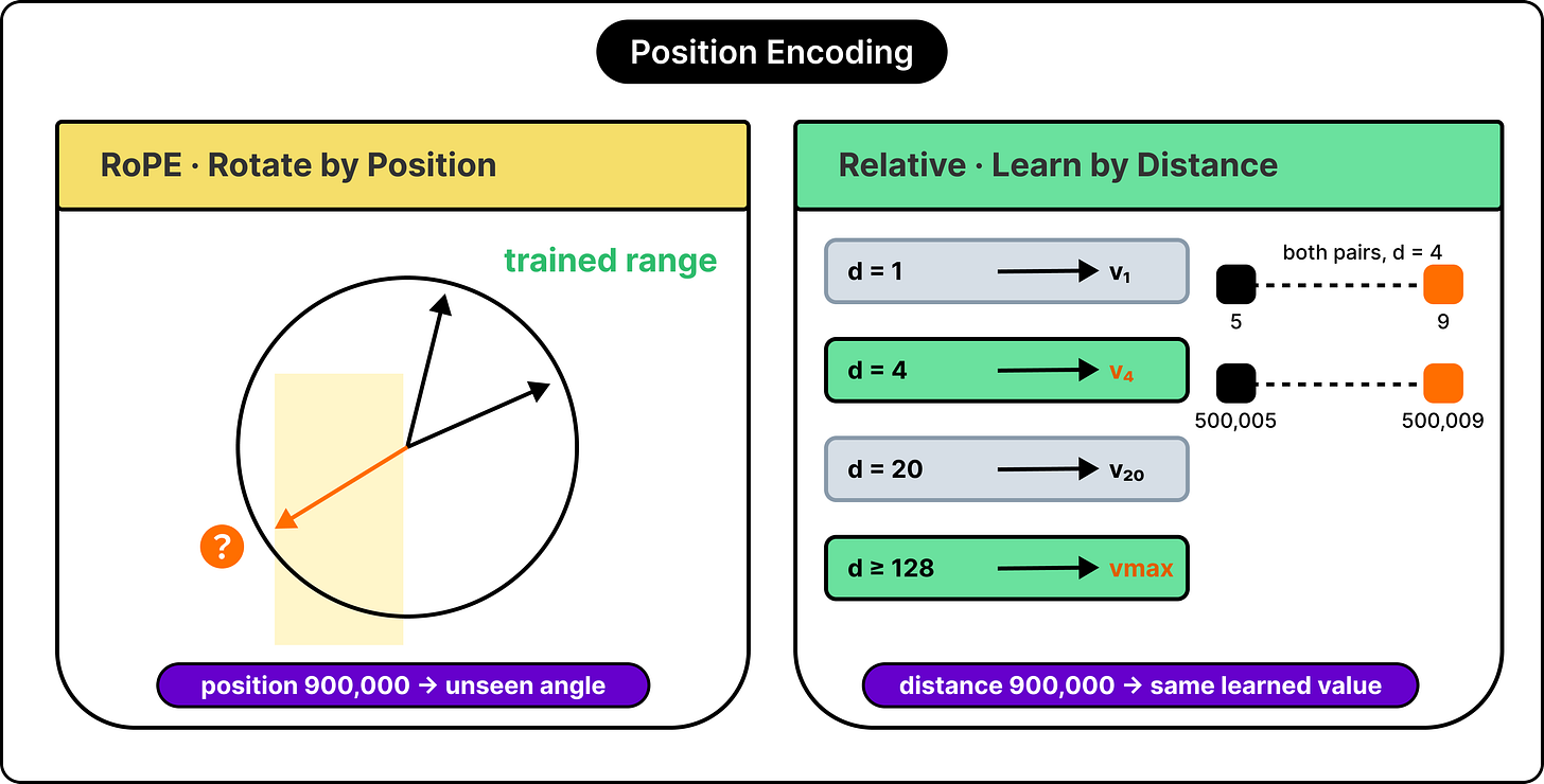
最近のオープンソースモデルのほとんどは、ロータリー・ポジション・エンベディング(RoPE)を採用しています。各トークンのクエリとキーは、そのトークンがシーケンス内のどこにあるかに比例した角度だけ回転する点として扱われます。1 番目のトークンはわずかな回転を受け、500 番目はより大きな回転を受け、というように続きます。
この手法の有用性は、2 つのトークンを比較する際に発揮されます。両方のトークンがそれぞれの位置に応じた量だけ回転しているため、その間の比較結果は二つの回転量の差に依存します。これが両者の距離を示すことになります。
しかし、これらの回転角度は、モデルが実際に学習した範囲でのみ出現しました。もし学習データが最大 32,000 トークンのシーケンスまでだった場合、モデルが解釈できるようになったすべての角度は、その範囲内からのものでした。900,000 番目の位置について問われた場合、関連する角度は学習経験の範囲を超えてしまいます。
RoPE を学習データを超える範囲に拡張するために、特定の技術群が存在します。
Inkling は、Shaw らの手法 [1][10] に基づく相対的な位置表現を採用しています。各トークンの絶対的な座標を符号化するのではなく、このアプローチでは 2 つのトークン間の距離ごとに学習された値を獲得し、それを比較スコアに直接加算します。
例えば、5 番目と 9 番目のトークンは 4 離れています。同様に、500,005 番目と 500,009 番目のトークンも 4 離れています。相対的な方式では、これら 2 つのペアは同じように扱われます。なぜなら、距離が「4」であれば、それがどこで発生しようとも同じ値だからです。
ある閾値(例えば 128)を超えた距離については、すべて共通の学習済み値を共有します。つまり、900,000 トークンも離れているペアに対しても、モデルはトレーニング中に何度も見たことのある値を使用します。外挿を行う必要はありません。
vLLM のノートでは、この実装がアテンションスコアを重みに変換する前に、学習された相対位置項を加えるものとして説明されています [7]。
Thinking Machines によると、この手法は RoPE(回転位置埋め込み)と比較して、より高い性能を発揮し、長いシーケンスへの外挿性も優れていました [1]。
Inkling は、アテンションが最初から学習しなければならない作業を処理するために、「畳み込み(convolution)」と呼ばれる小さな演算を追加しています。
ここで言う畳み込み(convolution)とは、シーケンス内の各位置を、その直前にある数個の位置と組み合わせる操作です。Inkling ではウィンドウサイズが 4 [7] に設定されており、100 番目の位置の数値は、97, 98, 99 番目の位置の数値と、少数の学習済み重みを用いて混合されます。同様に、101 番目の位置も 98, 99, 100 番目の位置と組み合わせます。これはコストが低く、固定された、厳密に局所的な操作です。
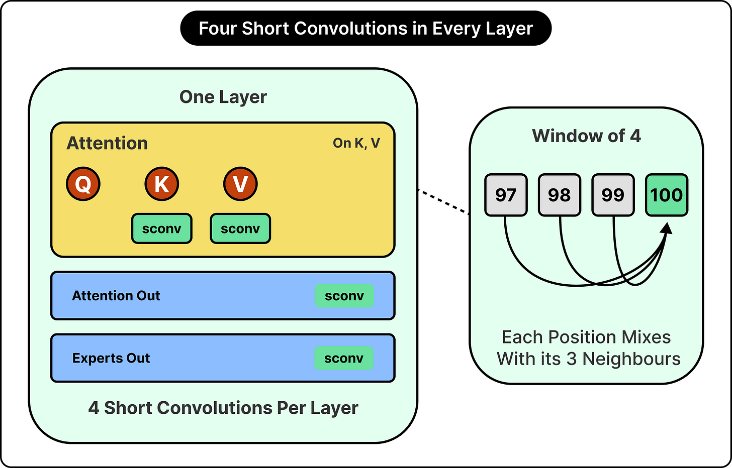
より深く理解するために、「New York」という 2 つのトークンを考えてみましょう。2 番目のトークンが単独で持つ意味は、1 番目のトークンの直後に続く場合とは大きく異なります。アテンション(attention)はこのつながりを学習できますが、その仕組みを学ぶ必要があります。なぜなら、アテンションは初期状態では近傍のトークンを遠くのトークンよりも優先する仕組みを持たない、一般的な比較メカニズムだからです。一方、畳み込みはその構造自体を通じて局所的な混合を直接提供し、隣接する要素が重要であることを学習するためのトレーニングを必要としません。
Thinking Machines は、これらの畳み込みを 2 つの種類の場所に配置しています:
- まず、各アテンション層内部にあるキーと値(keys and values)に対して
- 次に、アテンションおよびフィードフォワードステップの出力がモデル内のメインパスに再結合する前に、その出力に対して [1]。
原文を表示
AI coding agents can generate code quickly, but CI checks often happen after the agents finish their work. Sonar Vortex changes this pattern. Sonar Vortex operates inside the agent’s coding loop, giving agents architectural context before they write and verifying their output in real time as they produce it. Internal testing found 36% lower token consumption and 92% fewer defects.
Thinking Machines released a model called Inkling on July 15, 2026. A few interesting points made in its introduction are as follows:
- Inkling has 66 layers, and each layer holds 256 experts, of which only six activate for any given token [2].
- Most layers can access only a short window of recent text, while a few can access all of it [1].
- Word positions are encoded using a method most labs moved away from years ago.
Thinking Machines, founded by Mira Murati (the ex-CTO of OpenAI), describes its mission as building AI that extends human will and judgment. The company lists four directions of work, which are training strong models, building tools that let people customise models with their own knowledge, developing interfaces that widen the communication channel between people and machines, and publishing research on how models are made [3].
Before Inkling, the company shipped Tinker, a service for fine-tuning open models [4]. Inkling is the company’s first model trained from scratch [1]. The weights sit on Hugging Face under an Apache 2.0 license [2], so anyone can download them and retrain the model on their own data.
In this article, we will work through the various choices Thinking Machines made while building Inkling. Here is what we will cover:
- Mixture of Experts, and the gap between 975 billion parameters and 41 billion.
- The mix of local and global attention layers behind a context window of one million tokens.
- Position encoding, and the older method Thinking Machines chose over the current standard.
- How images and audio enter the model without a separately pretrained encoder in front of them.
- Thinking effort, a setting between 0 and 1 that adjusts how much the model reasons before answering.
*Disclaimer: This post is based on publicly shared details from various sources. References at the end. Please comment if you notice any inaccuracies.*
The diagram below shows where each of these five things sits inside the model.
Let us first understand four key terms that are really important to make sense of the architecture:
- Token: A token is a chunk of text. Models work with pieces smaller than sentences and usually a bit smaller than words. For example, the sentence “Inkling was released in July” might become six tokens, with common words getting one token each and unusual words getting split into two or three.
- Parameter: A parameter is one number stored inside the model, learned during training. When you read that a model has 975 billion parameters, it is the count of individual numbers sitting in the file. Each one started as random noise and was adjusted millions of times until the model produced sensible text.
- Training: It works by showing the model text, letting it predict the next token, comparing that prediction against the token that actually came next, and then adjusting every parameter slightly in whichever direction would have made the prediction better. The size and direction of each adjustment is called a gradient, and the procedure that computes all of them at once is called backpropagation. By repeating this across trillions of tokens, the parameters settle into values that produce useful predictions.
- Layer: It is one processing stage in the journey of a token. Inkling has 66 of them stacked in order [2]. A token’s representation enters layer 1, gets transformed, passes to layer 2, and so on until layer 66, after which the model predicts the next token. Every layer has the same two parts:An attention step that pulls in information from other tokens in the sequence.
- A feed-forward step that transforms the result.
Inkling separates the cost of storing a model from the cost of running it. This is the reason a model this large is affordable to use.
In an ordinary transformer, the feed-forward step in each layer is a single network, and every token passes through all of it. If that network holds 5 billion parameters, then every token processed involves all 5 billion.
Inkling replaces that single network with 256 smaller ones, called experts. For each token, a selection step picks six of the 256. Only those six run, and the remaining 250 sit idle for that token while handling other tokens instead [2]. This design pattern is called Mixture of Experts, and Thinking Machines states that their version largely follows the approach published by DeepSeek [1][8].
See the diagram below:
Let’s understand this via a simple example:
- Suppose you build a layer with 10 experts holding 1 billion parameters each, and you run 2 of them per token.
- The file on disk contains all 10 billion parameters, and every one of them has to be loaded into memory before you can run the model at all.
- Processing a single token involves 2 billion parameters, so each token costs about a fifth of what it would in an ordinary layer of the same total size.
Inkling does this at scale. The total across the whole model is 975 billion parameters, and the count involved in processing any single token is roughly 41 billion [1]. That is about 4 percent of the model running at a time.
The hardware requirements make things clearer. A checkpoint is the saved file holding all the trained parameters. Inkling’s full-precision checkpoint needs at least 2 TB of combined GPU memory, which the model card gives as eight NVIDIA B300 cards or sixteen H200 cards [2].
Thinking Machines also talks about a quantised checkpoint. This means the same parameters are stored with less numerical precision, in roughly the way that writing 3.14 instead of 3.14159265 uses less space at the cost of some accuracy. That version needs around 600 GB and fits on four B300 cards [2].
Strong candidates are skeptical of vague forward deployed engineer postings, and the title alone won’t earn their trust.
The free State of FDE Jobs 2026 Report explains what candidates look for, how the market is evolving, and how employers can make these roles easier to understand.
Hiring? You can also bring your openings to forwarddeployedengineer.com, the focused jobs board for forward-deployed engineers.
Picking six experts out of 256 sounds simple, but it is not. Here’s how the selection works:
- A small component called the router produces a score for every expert.
- Each expert has its own list of numbers attached to it, learned during training.
- The router compares the incoming token’s representation against each of those lists and gets a raw number out, higher when the two match closely.
- Those raw numbers can be any size, so they get passed through a sigmoid. A sigmoid is a mathematical function that takes any number and converts it into a value between 0 and 1. For example, feed it 8, and you get back about 0.9997. Feed it 0, and you get exactly 0.5. Feed it negative 4, and you get about 0.018. Very large numbers approach 1, very negative numbers approach 0, and everything else ends up somewhere in between. Inkling’s router uses a sigmoid to produce its expert scores [1].
- After scoring, the six highest-scoring experts run, and their outputs are combined using those same scores as weights. An expert scoring 0.9 contributes more to the result than one scoring 0.4.
This approach makes one specific type of failure more probable. To understand the failure, consider what happens across millions of training steps. Suppose, by luck, expert 47 gets picked slightly more often than average early on. It receives more tokens, so it receives more gradient updates, so it improves faster than its neighbours. Since it is better, the router scores it higher. Because it scores higher, it gets picked even more.
If we run that loop long enough, we can end up with a 256-expert layer where perhaps 20 experts handle nearly everything and the other 236 stay underdeveloped. This is called routing collapse. In other words, while we paid to store 256 experts, we got the capability of just 20. There is a second cost too. Since experts are usually spread across different machines, a machine holding four popular experts can become a bottleneck while its neighbours idle [9].
The traditional fix for this adds a penalty to the training objective that grows when expert usage is uneven. This means training the model on two things at once: predicting the next token correctly, and keeping expert usage balanced.
The trouble is that these two goals produce gradients pointing in different directions. The prediction gradient might say “increase this parameter,” while the balance penalty says “decrease it.” One of them wins, and either way the model is being pulled away from what you actually wanted. If we set the penalty strength high, the text quality degrades. If we set it too low, the experts collapse anyway [9].
Thinking Machines uses a method introduced by Wang and colleagues, which was also adopted by DeepSeek [1][8][9]. This method removes the conflict entirely by keeping a separate bias value for each expert, which is just a small number added to that expert’s score. The trick is where the bias gets applied.
Let us walk through a token arriving at a layer in this setup. Consider that the router produces these sigmoid scores for four of the experts.
Expert 47 has been overloaded recently, so its bias has drifted down to −0.15. This drops its selection score below expert 88’s, and expert 88 takes the slot instead. The bias changed which expert got picked. When expert 88’s output is combined into the final result, it is weighted by 0.80, its original router score, with the bias left out. In other words, the bias affects selection only. It never touches the weighting, and it is updated by a simple counting rule that runs outside backpropagation entirely. The main goal is to nudge down busy experts while giving a chance to the quieter experts.
The result is that expert usage stays balanced, and the training objective receives no competing gradient at all.
One point to note here is that two additional experts run on every single token regardless of routing [2]. These are called shared experts, and they hold the general-purpose processing that nearly every token needs. Thinking Machines states that the scores of the six selected routed experts and the two shared experts are normalised together before being used as weights [1], which means all eight are scaled to a common range and contribute proportionally. In other words, eight experts run per token in total.
Sparsity handles the cost of the feed-forward step. The attention step carries a separate cost that grows far faster, and Inkling manages it by having most layers examine very little.
For every token, the model computes three sets of numbers:
- A query, describing what kind of information this position needs.
- A key, describing what kind of information this position offers.
- A value, carrying the actual content this position passes along.
Every token’s query is compared against every earlier token’s key. Strong matches produce high scores, and those scores determine how much of each earlier token’s value gets pulled into the current position. This is how the word “it” in a sentence ends up connected to the noun it refers to.
Since every token compares itself against every earlier token, the number of comparisons grows with the square of the sequence length. For example:
- 1,000 tokens produce roughly 1 million comparisons.
- 10,000 tokens produce roughly 100 million.
- 1,000,000 tokens produce roughly 1 trillion.
Inkling supports a context window of one million tokens [2], and a trillion comparisons per layer across 66 layers is far beyond what any reasonable amount of hardware can deliver.
This is where a sliding-window layer restricts each token to a fixed number of recent tokens rather than everything before it. If the window is 1,000, then token number 500,000 compares itself against tokens 499,000 through 500,000 and stops there. That is 1,000 comparisons instead of 500,000, and the total for the whole sequence grows in a straight line rather than as a square.
This raises the obvious question that if every layer sees only a small window, how does information from page one of a long document ever reach page four hundred?
Inkling alternates between sliding-window layers and full-attention layers at a ratio of 5:1 [1]. Integration notes published by the vLLM project put concrete numbers on the split, describing the 66 layers as 55 sliding-window layers and 11 full-attention layers [7].
Information from far away travels through those eleven full layers. For example, picture a fact at token 200 that matters for a prediction at token 900,000. In layer 6, the first full-attention layer, the representation at position 900,000 can reach back and pick up that fact directly. From there, it rides forward within the local representations, is refreshed at layer 12, again at layer 18, and so on. The long-range path exists on roughly one layer in six, and the other five handle nearby context at a fraction of the price.
Inkling also uses 8 key-value heads [1]. Attention normally runs several times in parallel with different query, key, and value sets, and each parallel copy is called a head. Sharing a smaller number of key and value sets across many query heads reduces the memory needed while generating text.
See the diagram below that tries to show this setup in a simplistic manner:
There is one practical consequence of this approach. Long-context models often handle the general content of a large document well, but can still miss one specific detail buried in the middle.
Dealing with a million tokens brings up another question: how does the model represent where each token sits in the sequence?
Thinking Machines picked an older technique over the current standard. This is due to the lengths the model never saw during training.
The comparison between queries and keys involves no information about order. For example, both “the cat bit the man” and “the man bit the cat” contain the same five tokens, so without a position signal, the attention step produces the same comparisons for both. Something has to tell the model that “cat” came before “bit” in one case and after it in the other.
Almost every recent open model uses Rotary Position Embedding, shortened to RoPE. Each token’s query and key are treated as points that get rotated by an angle proportional to that token’s position in the sequence. Token 1 gets a small rotation, token 500 gets a much larger one, and so on.
The usefulness of this shows up when two tokens are compared. Since both were rotated by amounts tied to their own positions, the comparison between them depends on the difference between those two rotations, which tells how far apart they are.
However, those rotation angles were only ever encountered at positions the model actually trained on. If training used sequences up to 32,000 tokens, then every angle the model learned to interpret came from that range. If we ask it about position 900,000, the angle involved falls outside anything it has experience with.
A whole family of techniques exists specifically to stretch RoPE into ranges beyond its training data.
Inkling uses a relative scheme in the style of Shaw and colleagues [1][10]. Rather than encoding where each token sits, this approach learns a value for each distance between two tokens and adds that value directly to the comparison score. For example, tokens at positions 5 and 9 are 4 apart. Tokens at positions 500,005 and 500,009 are also 4 apart. A relative scheme treats both pairs identically, because 4 is 4 wherever it occurs. Distances beyond some cutoff, say anything more than 128 apart, all share the same learned value, so a pair 900,000 tokens apart uses a value the model has seen countless times during training. Nothing has to be extrapolated.
The vLLM notes describe the implementation as a learned relative-position term added to the attention scores before they are converted into weights [7].
Thinking Machines states that this performed better and extrapolated better to longer sequences than RoPE in their testing [1].
Inkling adds one small operation named convolution to handle a job that attention would otherwise have to learn from scratch.
A convolution here means combining each position in the sequence with a few positions immediately before it. Inkling uses a window of four [7], so the numbers at position 100 get mixed with the numbers at positions 97, 98, and 99, using a small set of learned weights. Position 101 does the same with 98, 99, and 100. It is a cheap, fixed, strictly local operation.
To understand better, consider the two tokens that make up “New York.” The second token means something quite different on its own than it does following the first. Attention can learn to make that connection, and it has to learn it, because attention starts as a general comparison mechanism with no built-in preference for nearby tokens over distant ones. A convolution supplies that local mixing directly through its structure, without any training required to discover that neighbours matter.
Thinking Machines places these convolutions at two kinds of locations:
- First, on the keys and values inside each attention layer
Second, on the outputs of the attention and feed-forward steps before those outputs rejoin the main path through the model [1].
今日のまとめ
AIデイリーブリーフで今日の重要ニュースをまとめ読み