Amazon SageMaker AI エンドポイントの推論メタモニタリング
AWS は Amazon SageMaker AI エンドポイント向けの推論メタモニタリング機能を導入し、モデルの品質低下やデータドリフトを継続的に追跡・可視化するガバナンス層を提供する。
AI深層分析を開く2026年7月31日 02:14
AI深層分析
キーポイント
推論モニタリングのギャップ解消
顧客からの苦情や点検まで待たずに、モデルのパフォーマンスが静かに劣化している問題を早期に検知できる必要性を指摘し、その解決策としてメタモニタリングの重要性を説く。
AWS 管理サービスとオープンソースツールの統合
Amazon SageMaker AI、Athena、Lambda、EventBridge、Quick を中心に、SageMaker AI MLflow App や Evidently AI と組み合わせたハイブリッドな監視ソリューションを提案する。
包括的な機能構成
ドリフト検知、遅延する正解データの統合、自動化されたパフォーマンスダッシュボードを含むシステム設計により、予測モデルの品質とデータ品質を継続的に追跡する仕組みを提供する。
実装のための要件と手順
AWS アカウントの準備や CloudFormation テンプレートを使用した VPC 構築など、具体的な実装に必要な前提条件と初期設定の手順を提示する。
CloudFormationテンプレートによるセットアップ自動化
提供されたCloudFormationテンプレートを使用すると、VPC、サブネット、SageMaker AIドメインなどのリソースが自動的に作成され、.envファイルが実際の値に更新される。既存のドメインを利用する場合は、リポジトリをクローンして.envファイルを編集し、ノートブックを順次実行することで設定が可能である。
重要な引用
Without the ability to track machine learning (ML) model prediction quality, organizations only realize they have issues when their customers complain or when they conduct spot checks, which jeopardizes customer trust.
The performance of the models you deploy might silently degrade, and your teams might notice it only weeks later.
This inference meta-monitoring solution combines AWS managed services with open source ML tools.
The system implements integrated training, inference, and monitoring pipelines, unified through a central Athena Iceberg table, Amazon Quick and SageMaker AI MLflow Apps.
編集コメントを表示
編集コメント
AWS は推論段階のモデル品質管理において、単なる監視を超えたガバナンス機能の提供を強化している。このアプローチは、大規模な ML プロジェクトにおける運用リスクを低減し、信頼性の高い AI サービス展開を支援する重要な一歩となる。
Source Article
元記事を日本語で読む
本文に関係しない購読案内、埋め込み通知、サイト内プロモーションは除いています。
機械学習(ML)モデルの予測品質を追跡する手段がなければ、組織は顧客からの苦情や不意打ちの点検が行われるまで問題に気づくことができません。これは顧客信頼を損なうリスクがあります。
本記事では、Amazon SageMaker AI エンドポイント向けの推論メタモニタリングについて紹介します。これは、生産環境での ML 推論パイプラインの上に位置するガバナンス層であり、予測品質とデータ品質の指標を継続的に追跡し、その傾向を可視化します。
ここでは、Amazon QuickSight を使用して(必要に応じて Amazon SageMaker AI MLflow App と併用)、予測モデルに特化した推論メタモニタリングシステムの設計と実装方法を解説します。このシステムには、ドリフト検出機能、遅延する正解データ(ground truth)の統合、および自動化されたパフォーマンスダッシュボードが含まれています。
推論モニタリングのギャップ
予測 ML モデルの開発は、往々にしてリソースを大量に消費するプロセスです。不正検知、与信スコアリング、需要予測といったユースケースで高い検証精度を達成するために、訓練パイプラインの構築に数ヶ月を費やします。
しかし、デプロイしたモデルのパフォーマンスが静かに低下しても、チームがそれに気づくのは数週間後になるかもしれません。不正案件処理担当者は誤検知(false positives)の急増に直面し、融資担当者は以前ならフラグが立っていたはずの申請が増えていることに気づきます。また、企業資源計画(ERP)担当者たちは、需要予測の過大評価によって在庫過多という問題を抱えることになります。
ML チームには、本番環境でのモデルパフォーマンスに関する継続的なフィードバックを提供するシステムが必要です。このシステムは、モデルの品質低下やデータドリフトを検知した際に即座にアラートを発令し、チームが早期に対応できるようにする必要があります。これにより、時間経過に伴うモデルパフォーマンスの一貫性を維持し、顧客からの信頼を高めることが可能になります。
ソリューション概要
本インフラメタモニタリングソリューションは、AWS のマネージドサービス(Amazon SageMaker AI、Amazon Athena、AWS Lambda、Amazon EventBridge、Amazon QuickSight)とオープンソースの ML ツール(SageMaker AI MLflow Apps、Evidently AI)を組み合わせています。
事前要件
- AWS アカウントが必要です。
- リポジトリ内の CloudFormation テンプレートを使用して、仮想プライベートクラウド(VPC)、サブネット、SageMaker AI ドメイン、ユーザープロファイル、JupyterLab スペースを作成します。テンプレートはまた、Git リポジトリをクローンし、.env ファイルに実際の値を反映させて更新します。
セットアップ
CloudFormation テンプレートによりセットアップ全体が自動化されます。既存のドメインを利用する場合は、リポジトリをクローンして環境変数の値を更新し、ノートブックを順次実行してください。
環境設定
CloudFormation のセットアップを実行すると、必要な変数が作成され初期化されます。
独自の SageMaker AI ドメインを利用する場合は、.env.example ファイルを .env としてコピーし、環境変数を自身の設定に合わせて更新してください。.env ファイルの設定は、他のすべてのデフォルト値や config.yaml の設定を上書きします。
git clone --branch v2.0.0 https://github.com/aws-samples/sample-mlops-bestpractices.git
cd sagemaker-automated-drift-and-trend-monitoring
cp .env.example .env
アーキテクチャ
本システムは、中央の Athena Iceberg テーブルと Amazon QuickSight、SageMaker AI MLflow アプリを中核に据え、トレーニング、推論、モニタリングのパイプラインを統合しています。
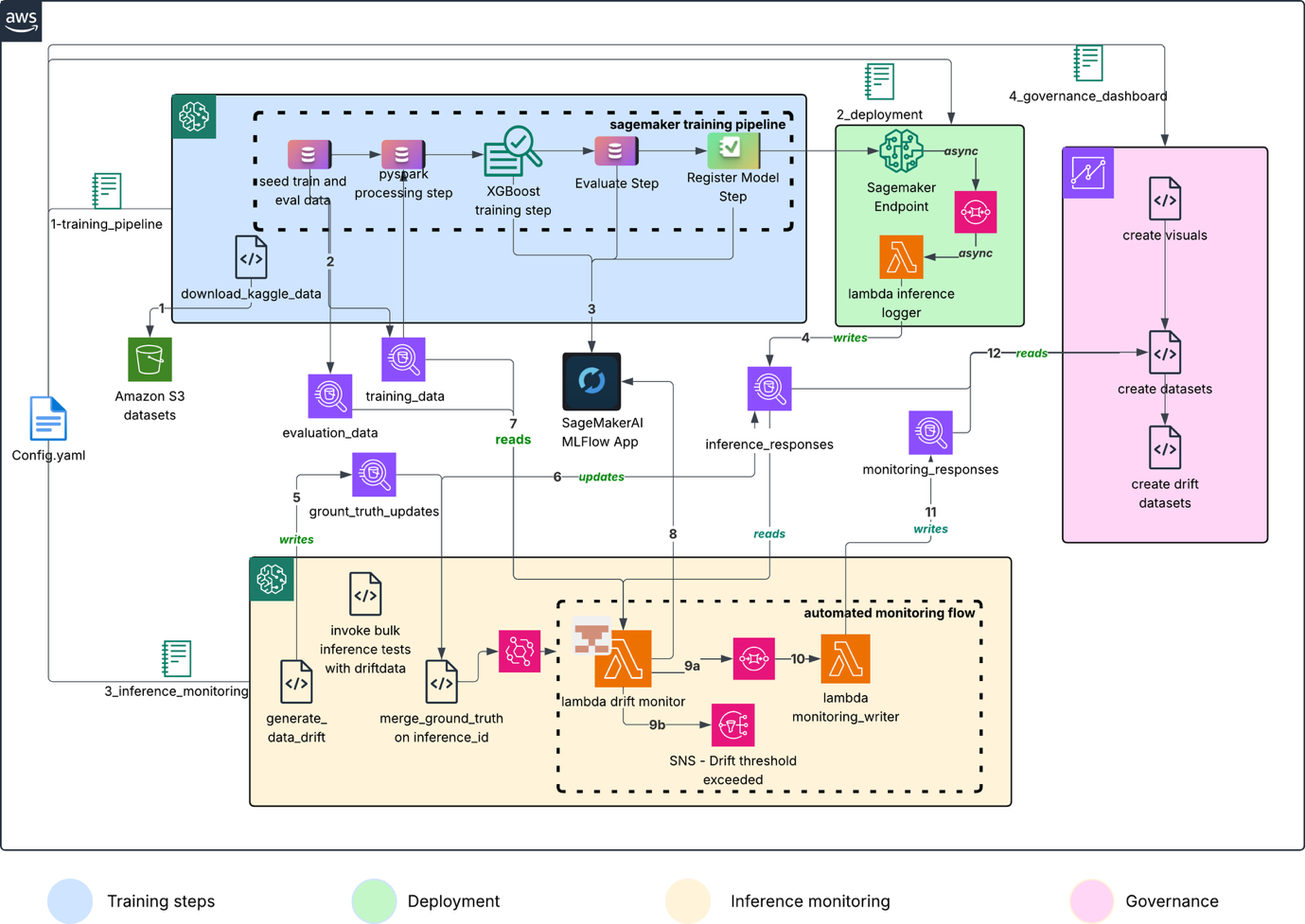
図 1: AWS マネージドサービスで構築されたエンドツーエンドの MLOps アーキテクチャ
トレーニング (1_training_pipeline.ipynb)
トレーニングパイプラインには MLflow を用いた実験追跡機能が組み込まれています。図 2 に示す通り、これはモデルの学習から推論までの一連のプロセスを構築するものです。
- Kaggle データセットのダウンロード: クレジットカード不正検出データセット を Kaggle から取得します。
- データの取り込み:S3 に保存されたデータはトレーニング用データとして読み込まれます。本アーキテクチャでは、5 つの Athena Iceberg テーブルを中核に据えたデータレイクを構築しています。
training_data テーブルにはモデル学習に使用するデータの 80% が格納され、evaluation_data テーブルには評価用の 20%(ホールドアウトデータ)が保存されます。ドリフト監視の基準となるのは training_data ではなく evaluation_data です。なぜなら、登録されたすべてのモデルの評価指標は、この固定されたホールドアウトスライスに対して測定されるからです。
両テーブルとも、同じ予測結果 CSV ファイルから単一のシードステップによって作成されます。この際、transaction_id を鍵とした決定論的なハッシュ分割が行われるため、パイプラインの実行ごとにデータ行の割り当てが安定します。
図 2 に示す「SeedAthenaTrainingData」ステップでは、transaction_id による決定論的なハッシュ分割を用いて、S3 から予測結果 CSV を読み込み、これを training_data(80%)と evaluation_data(20%)の Iceberg テーブルに重複実行可能な形でロードします。再実行しても行の割り当ては同一となるため、評価用スライスはモデルバージョン間でも安定しており、ドリフト監視のための固定基準として利用可能です。
必要に応じてトレーニングデータ自体を独自のデータに置き換えることもできます。詳細については、Bring your own dataset をご参照ください。
- トレーニング:トレーニングと評価のステップは実行され、その結果として得られるメトリクスやアーティファクトは、SageMaker AI MLflow App にログ出力されます。
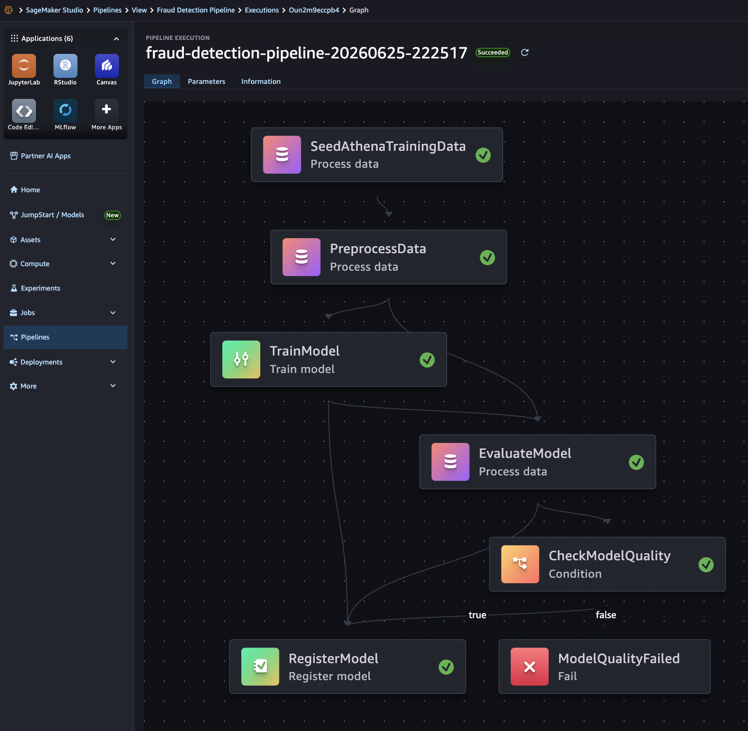
Figure 2: Training pipeline execution
Model deployment (2_deployment.ipynb)
4. デプロイ: カスタムハンドラーを SageMaker AI の推論エンドポイントにデプロイします。
推論ハンドラーは、すべての推論結果を Amazon Simple Queue Service(Amazon SQS)へ書き出します。その後、推論ログ記録用の Lambda 関数がこれらを受信処理します。この Lambda 関数は、最大 10 件の予測、または 30 秒以内に到着した予測の数(いずれか早い方)をバッチ化し、Athena Iceberg テーブルへ書き込みます。
すべてのノートブックには、ロール作成やインフラストラクチャ構築のためのユーティリティスクリプトも含まれています。
Inference monitoring (3_inference_monitoring.ipynb)
5. 正解値のシミュレーション: 3_inference_monitoring.ipynb の手順 3.3 では、ドリフトした入力特徴量を用いてデプロイ済みモデルを呼び出します。これによりデータドリフトが発生します。
実際の運用環境では、これは時間経過とともにドリフトした入力で推論リクエストを送信する一般的なビジネスアプリケーションに相当します。正解値のシミュレーションはノートブック内の手順 4 に該当します。
本ソリューションの手順 3 と 4 は、データドリフトやモデルドリフトの計算を行う前に実行される自社の業務プロセスに置き換えることを想定しています。
a. ステップ 3: アプリケーションが推論エンドポイントにリクエストを送信します。これにより、推論エンドポイントから SQS へ、次に Lambda を経由して Athena(inference_responses)へ推論リクエストがプッシュされます。
b. ステップ 4: グラウンドトゥルースデータの生成を行います。これは予測が正しかったか間違っていたかを判定するプロセスです。今回のユースケースでは、推論リクエストが不正(fraud)だったのか正常(non-fraud)だったのかを判断します。本ソリューションでは、モデルの性能に 15% の不正確さを意図的に含めるため、実際のフィールド値をランダムに「不正」または「正常」に反転させるシミュレーションを行います。これによりモデルドリフトが発生します。実世界のシナリオでは、自動承認された取引や顧客による請求取り消し(チャージバック)、あるいは銀行からの確認に基づき、不正調査チームがラベルを検証・確定した時点で、実際の不正/正常の判定が行われます。
注記:ノートブック 3 のステップ 2、3、4(ドリフトデータの生成、予測の送信、グラウンドトゥルースの適用)はスケジュールされた操作ではありません。これらは開発およびテスト目的のために用意されたものです。本番環境では、これらの手順を自社のビジネスプロセスに置き換える必要があります。具体的には、推論のためにエンドポイントにアクセスするアプリケーション(ステップ 2〜3)と、グラウンドトゥルース更新(ground_truth_updates)へデータを書き込む不正調査フィード(ステップ 4)です。本ソリューションをエンドツーエンドで試す場合は、リポジトリ内のノートブックセルまたは CLI スクリプトを使用して、これら 3 つのステップを手動でトリガーしてください。
ステップ 2 と 3 を完了すると、データドリフトを検知した推論リクエストはすでに inference_responses テーブルに格納されています。次にステップ 4 では、ground_truth_updates テーブルへレコードが書き込まれます。ここでは ground_truth が NULL のレコードを抽出し、実際のラベルを用いて新しいレコードを作成します。これにより、計算処理を通じてモデルドリフトの検出が可能になります。
任意のタイミングで、お好みのクエリエディタを使用してレコードを検証できます:
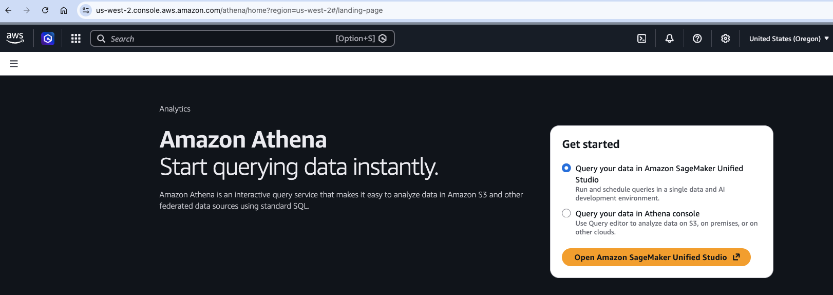
図 3:生成されたレコードを表示するクエリエディタ
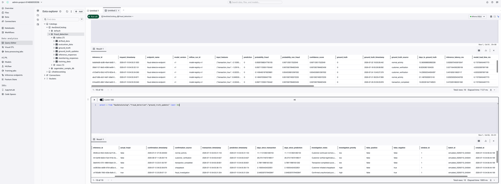
図 4:ground_truth の更新情報を反映した inference_responses テーブルと ground_truth_updates テーブル内のレコード
inference_responses テーブルにおいて、ground_truth が NULL のレコードは、まだ正解ラベルが適用されていないエントリに対応しています。
6. グランドトゥルースと推論応答の統合
inference_responsesテーブルに記録された予測値や推論リクエストは、ground_truth_updatesテーブルとinference_idで結合できます。inference_responsesテーブルには、各予測に対応する特徴量、信頼度スコア、タイムスタンプがすべて記録されます。一方、ground_truth_updatesテーブルには非同期のラベル確認情報が格納されており、これらは手順4を通じて推論レコードにマージされます(詳細はノートブックを参照)。
これでデータドリフトとモデルドリフトの計算に必要なデータが揃ったため、両方のカテゴリにおけるベースラインおよび現在のデータを特定できます。以下にその構成を示します。
| メトリック | コンポーネント | ソース | ID | 設定 | 例 |
|---|---|---|---|---|---|
| データドリフト | ベースライン | training_data | Icebergテーブルのsnapshot_id(baseline.jsonにも記録) | プリプロセスステップで自動取得 | 訓練データの取引金額の平均が$50だった場合でも、直近の予測値の平均が$500に達した場合、KS検定により分布のシフトとしてフラグが立ちます。 |
| | 現在 | lookbackウィンドウ内のinference_responses | リクエストタイムスタンプがローリング時間窓より後のレコード | ドリフト用Lambda環境変数:
DATA_DRIFT_LOOKBACK_DAYS: 1 # 過去1日分の推論を照会
DATA_DRIFT_THRESHOLD: 0.2 # 特徴量の20%以上がドリフトした場合にアラート |
モデルドリフト
ベースライン評価データには、Iceberg テーブル内の Snapshot ID が記録されており、これは baseline.json にも併せて保存されます。このプロセスは前処理ステップ中に自動的に実行されます。
Lambda は過去 30 日間の予測データを取得し、正解ラベル(ground truth)が存在するものだけを抽出します。そして現在の ROC-AUC を計算します。例えば、ベースラインが 0.92 で現在の値が 0.85 の場合、ROC-AUC の低下幅は 0.07 となります。これは設定された閾値 0.05 を超えているため、アラートが発令されます。
現在の監視では、ローリングウィンドウ内のリクエストタイムスタンプを持つ Inference_responses レコードが対象となります。
ドリフト計算用の Lambda 環境変数として MODEL_DRIFT_LOOKBACK_DAYS が設定されています。デプロイスクリプト(deploy_lambda_container.sh)では、Lambda の実行スケジュールが日次であるため、この値は「1」に設定されます。ただし、ビジネスプロセス上で正解ラベルがどの程度遅れて到着するかによって、この期間を調整する必要があります。なお、ノートブック駆動のフロー用として用意された config.yaml のデフォルト値は 30 日です。これは正解ラベルが遅れることが多いため、より長いウィンドウを設定する必要があるからです。
注意: ドリフト計算のために短いウィンドウ(分単位)を使用したい場合は、Configuring Shorter Drift Windows (Minutes instead of days) の手順に従ってください。
monitoring_responses テーブルには、ドリフト計算の結果が格納されます。これには、モデルパッケージの ARN や計算対象となった Iceberg のスナップショット ID が含まれており、モデルバージョンごとにトレンドを切り分けて分析することが可能になります。
登録されたモデルには、評価データにおけるスコアや、そのデータスライスの Iceberg スナップショット ID、そして生成時のコードコミット SHA を記録した「frozen baseline.json」アーティファクトが必ず含まれています。ドリフト検出用の Lambda は実行ごとにこれらのポインタを参照するため、監視システムは常に本番環境と、デプロイされたモデルの元となった正確なデータおよびコードバージョンを比較します。これにより、古い情報や誤ったバージョンへの言及が一切発生しないよう保証されます。詳細な系譜(ラインージ)メカニズムについては、後述する深掘りセクションで解説しています。
7. ドリフト計算: ドリフト検出用の Lambda 関数は、エンドポイントで現在提供されているモデルを特定し、登録された baseline.json を読み込みます。各呼び出しでは 2 つの独立したチェックが実行され、それぞれが独自の凍結済みベースラインに対して評価されます。
データドリフトについては、baseline.json の training_snapshot_id で固定されたトレーニングデータの断片(スライス)が、モデル学習時の参照分布となります。一方、ローリングウィンドウ内の最新の inference_responses.input_features が現在の分布です。Evidently の DataDriftPreset がこれら 2 つを比較し、各列に対して自動的に統計検定を選択します。サンプルサイズが小さい場合は Kolmogorov-Smirnov 検定またはカイ二乗検定(p 値)を使用し、n が 1000 以上の場合は Wasserstein 距離や Jensen-Shannon 距離を採用します。
モデルドリフトについては、evaluation_snapshot_id で固定された評価データの断片がベースラインとなります。これは学習時にモデルの評価に使用された(ターゲットと予測の)ペアです。現在の推論行を ground_truth_updates と結合し、Evidently の ClassificationPreset を用いてこのベースラインと比較します。ClassificationPreset は、ROC-AUC、精度、再現率、F1 スコアの低下を追跡します。
両方のベースラインはモデルバージョンごとに不変であるため、後からソーステーブルを再シードしても、過去のドリフト比較結果が書き換わることはありません。Evidently が出力する生スコアは選択した検定方法によってドリフトの方向性が異なる(p 値の場合は低いほどドリフト、距離の場合は高いほどドリフト)ため、本ソリューションではさらに drift_magnitude という正規化された補完フィールドも計算しています。これにより、どの検定手法を使用しているかに関わらず特徴量を比較・順位付けすることが可能になります。
詳細なメトリクスについては、drift story を参照してください。
注意:2 つの追加テーブルが作成されますが、現在は未使用です。ground_truth テーブルには確認済みのラベル(不正/正常)が格納され、モデル再学習時にベースラインデータに追加データを反映させるためのプレースホルダーとして確保されています。また、drifted_data テーブルも必要に応じてドリフトしたデータセットを格納するためのプレースホルダーとして作成されます。
8. ドリフトのログ記録: ドリフト監視 Lambda 関数は Evidently を使用して対話型チャートを生成し、SageMaker AI MLflow App にログ出力します。また、すべての分析に Amazon QuickSight のみを指定することも可能です。本ソリューションは、データサイエンティストとガバナンス担当者の両方のニーズに対応するため、Evidently と連携した MLflow および Amazon QuickSight の双方をサポートしています。
9. モニタリングの自動化: ドリフト監視 Lambda 関数はドリフト閾値をチェックし、閾値を超えた場合にアラームをトリガーします。
10 – 11. ドリフト監視 Lambda 関数は計算結果を Amazon SQS にプッシュし、Lambda Writer がその結果を読み取って monitoring_responses テーブルに出力を書き込みます。本ソリューションでは Apache Iceberg ベースの Athena テーブルを使用しているため、更新処理は ACID 準拠となっています。
メタモニタリング(
原文を表示
Without the ability to track machine learning (ML) model prediction quality, organizations only realize they have issues when their customers complain or when they conduct spot checks, which jeopardizes customer trust. This post introduces inference meta-monitoring for Amazon SageMaker AI endpoints. It provides a governance layer that sits above production ML inference pipelines to continuously track prediction and data quality metrics and visualize trends. You will learn how to design and implement an inference meta-monitoring system specifically for predictive models, using Amazon Quick and optionally with Amazon SageMaker AI MLflow App. The system includes drift detection, delayed ground truth data integration, and automated performance dashboards.
The inference monitoring gap
Developing predictive ML models is often a resource-intensive process. You invest months building training pipelines to drive strong validation accuracy for use cases such as fraud detection, credit scoring or demand forecasting. The performance of the models you deploy might silently degrade, and your teams might notice it only weeks later. Fraud case handlers start to see false positives spiking, and loan officers start to see more applications that should have been previously flagged. Corporate resource planners find themselves with excess inventory because of overestimated demand forecasts.
ML teams therefore need a system that provides them with continuous feedback on the performance of their models in production. The system should immediately alert them whenever model quality or data drift is detected. Teams can then take action early so that model performance remains consistent over time, and customer trust remains high.
Solution overview
This inference meta-monitoring solution combines AWS managed services (Amazon SageMaker AI, Amazon Athena, AWS Lambda, Amazon EventBridge, Amazon Quick) with open source ML tools (SageMaker AI MLflow Apps, Evidently AI).
Prerequisites
- AWS account.
- Use the CloudFormation template provided in the repo to create the virtual private cloud (VPC), subnets, SageMaker AI domain, user profile, and JupyterLab space. The template also clones the git repo and updates the .env with the actual values.
Setup
The CloudFormation template automates the entire setup. If you intend to use your existing domains, you can clone the repository, update the env values and run the notebooks in sequence.
Environment setup
Running the CloudFormation setup creates and initializes the variables.
If you intend to use your own SageMaker AI domain, copy over the .env.example to .env and update the file with your specific environment variables. The settings in .env override all other defaults and settings in config.yaml.
git clone --branch v2.0.0 https://github.com/aws-samples/sample-mlops-bestpractices.git
cd sagemaker-automated-drift-and-trend-monitoring
cp .env.example .envArchitecture
The system implements integrated training, inference, and monitoring pipelines, unified through a central Athena Iceberg table, Amazon Quick and SageMaker AI MLflow Apps.
Figure 1: End-to-end MLOps architecture built on AWS managed services
Training (1_training_pipeline.ipynb)
The training pipeline includes experiment tracking in MLflow. As shown in Figure 2, it sets up the end-to-end model training.
- Download Kaggle dataset: Credit card fraud dataset is downloaded from Kaggle.
- Data ingestion: S3 data is loaded into the training data. The architecture uses five Athena Iceberg tables to form the central data lake. The training_data table stores the 80% slice the model is fit on. The evaluation_data table is the frozen 20% held-out slice the model is scored on. evaluation_data is the drift-monitoring baseline, not training_data, because the held-out slice is what every registered model’s metrics are measured against. Both tables are populated from the same predictions CSV by a single seed step that applies a deterministic hash split on transaction_id, so the row partition is stable across pipeline runs.
The SeedAthenaTrainingData step (see Figure 2) idempotently loads the predictions CSV from Amazon S3 into the training_data (80%) and evaluation_data (20%) Iceberg tables using a deterministic hash split on transaction_id. Re-runs produce identical row partitions, so the evaluation slice is stable across model versions and usable as a frozen drift baseline. Alternatively, you can replace the training data with your own. For further details, refer to Bring your own dataset.
- Training: The training and evaluation steps run and log metrics and artifacts to a SageMaker AI MLflow App.
Figure 2: Training pipeline execution
Model deployment (2_deployment.ipynb)
4. Deployment: A custom handler is deployed to a SageMaker AI inference endpoint.
The inference handler writes all the inferences to Amazon Simple Queue Service (Amazon SQS), which are then processed by an inference-logger Lambda function. The inference-logger Lambda function batches up to 10 predictions, or the number of predictions that arrive within 30 seconds, whichever comes first, and writes into Athena Iceberg tables. All the notebooks also include convenience scripts for role creation and infrastructure creation.
Inference monitoring (3_inference_monitoring.ipynb)
5. Ground truth simulation: Step 3.3 in 3_inference_monitoring.ipynb invokes the deployed model with drifted input features. This infuses data drift. In real environments, this would be your typical business applications that send inference requests with drifted inputs over time. The ground truth simulation is step 4 in the notebook.
Steps 3 and 4 of the solution are meant to be replaced by your business processes, which perform two steps before the data and model drift computations:
a. Step 3: Your applications invoke the endpoint for inference. This triggers the inference endpoint to push the inference request into SQS -> Lambda -> Athena (inference_responses).
b. Step 4: You generate ground truth data. This is the process of concluding if a prediction was right or wrong. In the example use case, it is determining if an inference request was a fraud or non-fraud. In this solution, the ground truth simulation randomly flips the actual field to be fraud/non-fraud, to infuse 15% inaccuracy in model performance. This induces model drift. In real-world scenarios, the actual fraud/non-fraud designation would be made when your fraud team investigates and confirms labels based on auto-approved transactions, customer-disputed chargebacks or a bank confirming fraud/non-fraud cases.
NOTE: Steps 2, 3, and 4 in notebook 3 (generate drifted data, send predictions, apply ground truth) are not scheduled operations. They exist only for dev/test purposes. In production you would replace these with your own business processes: applications hitting the endpoint for inference (steps 2-3) and fraud-investigation feeds writing to ground_truth_updates (step 4). To try this solution end-to-end, trigger these three steps via the notebook cells or the CLI scripts provided in the repo.
With steps 2 and 3, inference requests with data drift are already in inference_responses. Step 4 writes records into the ground_truth_updates table. Records with ground_truth = NULL are picked and new records are created in the ground_truth_updates table with actual labels. With this we can expect model drift upon computation.
At any point you can validate the records through a query editor of your choice:
Figure 3: Query editor showing the generated records
Figure 4: Records in the inference_responses table with ground truth updates and the ground_truth_updates table
Records in the inference_responses table with ground_truth=NULL correspond to the entries for which ground truth hasn’t been applied.
6. Merge ground truth with inference response: Predictions and inference requests captured in the inference_responses table can be joined with ground_truth_updates on inference_id. The inference_responses table captures every prediction along with its features, confidence scores, and timestamps. The ground_truth_updates table holds asynchronous label confirmations that are merged back into inference records through step 4 in the notebook.
Now that we have data to compute data and model drift, we can identify the baseline and current datasets for both categories of computations:
Metric
Component
Source
ID
Configuration
Example
Data Drift
Baseline
training_data
Snapshot_id in iceberg_table also recorded in baseline.json
Automatic during preprocessing step
If training data had transaction_amount with mean=$50, but recent predictions
show mean=$500, KS test would flag this distribution shift.
Current
Inference_responses for the lookback window
records where request_timestamp >= rolling time window
Drift lambda env var:
DATA_DRIFT_LOOKBACK_DAYS: 1 # Query last 1 days of inferences
DATA_DRIFT_THRESHOLD: 0.2 # Alert if ≥20% features drifted
Model drift
Baseline
Evaluation_data
Snapshot_id in iceberg_table and also recorded in baseline.json
Automatic during preprocessing step
Lambda queries predictions from last 30 days that have ground truth labels,
calculates
Lambda queries predictions from last 30 days that have ground truth labels, calculates current ROC-AUC. If baseline was 0.92 and current is 0.85, ROC-AUC degradation = 0.07 (exceeds 0.05 threshold) → Alert!
0.05 threshold) → Alert!
Current
Inference_responses with
records where request_timestamp >= rolling time window
Drift lambda env var:
MODEL_DRIFT_LOOKBACK_DAYS: 1 – set to 1 day in deploy_lambda_container.sh because the Lambda is on a daily schedule. Change this value based on how quickly ground truth arrives in your business processes. The config.yaml default is 30 days (for the notebook-driven flow, where a longer window is appropriate because ground truth is often delayed).
Note: If you intend to have a shorter window for drift computations, follow the steps detailed in Configuring Shorter Drift Windows (Minutes instead of days)
The monitoring_responses table stores outputs from the drift computations, including the ModelPackage ARN and Iceberg snapshot ID the run was computed against, so trends can be sliced per model version.
Every registered model carries a frozen baseline.json artifact that records the metrics it earned on evaluation_data, the Iceberg snapshot ID of that exact data slice, and the code commit SHA that produced it. The drift Lambda dereferences these pointers on every run, so the monitoring system always compares production against the precise version of the data and code the deployed model came from, ensuring there is never a stale or wrong-version reference. The lineage mechanism is described in detail in the deep dive section that follows.
7. Drift computation: The drift Lambda function resolves the model currently served by the endpoint and loads its registered baseline.json. Two independent checks run on each invocation, each against its own frozen baseline. For data drift, the frozen training_data slice (pinned through training_snapshot_id in baseline.json) is the reference distribution the model was trained on. Recent inference_responses.input_features from the rolling window is the current distribution. Evidently’s DataDriftPreset compares the two, auto-selecting a statistical test per column. It uses the Kolmogorov-Smirnov or Chi-square (p-values) for smaller samples, and Wasserstein or Jensen-Shannon distances for n ≥ 1000. For model drift, the frozen evaluation_data slice (pinned through evaluation_snapshot_id) supplies the baseline (target, prediction) pairs the model was scored on at training time. Current inference rows joined with ground_truth_updates are compared to that baseline via Evidently’s ClassificationPreset, which tracks ROC-AUC, precision, recall, and F1 degradation. Both baselines are immutable per model version, so re-seeding the source tables later cannot retroactively change historical drift comparisons. Because Evidently emits raw scores whose drift direction depends on the chosen test (p-values: lower = drift. Distances: higher = drift), the solution also computes a normalized companion field, drift_magnitude, so features can be compared and ranked test-agnostically. Follow the drift story for deeper insight into the metrics.
NOTE: Two additional tables are created but not currently used. The ground_truth table holds confirmed labels (fraud/not fraud) and is reserved as a placeholder to update the baseline data for cases where the model has been retrained and you would like to add additional data to the baseline. The drifted_data table is created as a placeholder to contain drifted datasets if needed.
8. Drift logging: The drift monitor Lambda function uses Evidently to generate interactive charts which get logged to SageMaker AI MLflow App. You can also choose to use only Amazon Quick for all your analytics. This solution provides both MLflow with Evidently and Amazon Quick support to cater to both data scientists and governance personas.
9. Monitoring automation: The drift monitor Lambda function checks drift thresholds and triggers alarms if the thresholds are exceeded.
10 – 11. The drift monitor Lambda function also pushes the computations to Amazon SQS and the Lambda writer reads the results and writes the output to the monitoring_responses table. Since the solution uses Apache Iceberg based Athena tables, updates are ACID-compliant.
Meta-monitoring (
AI算出
技術分析ainew評価標準
推論メタモニタリングという AI/ML 運用の重要な課題に焦点を当て、SageMaker と QuickSight を用いた具体的な設計・実装方法を詳述しており技術分析として適切です。ただし、これは既存ツールの組み合わせによるベストプラクティスの紹介であり、世界初の新機能発表や独自データに基づく市場分析ではないため、新規性と日本固有の価値は低めに見積もります。
6つの評価軸を見る
- AI関連度
- 75
- 情報源の信頼性
- 100
- 新規性
- 25
- 調べる価値
- 75
- 重複の少なさ
- 100
- 日本での有用性
- 25
関連記事
今日のまとめ
AIデイリーブリーフで今日の重要ニュースをまとめ読み