LLM アーキテクチャの最近の動向:KV シェアリング、mHC、圧縮アテンションについて
Sebastian Raschka は、長文コンテキスト処理における効率化を目的とした、KV キャッシュ共有や圧縮アテンションなど、最新のオープンウェイト LLM アーキテクチャの具体的な技術的進展と設計思想を詳細に分析している。
キーポイント
長文コンテキスト処理のボトルネック解消への注力
推論モデルやエージェントワークフローにおいてトークン数が長期化・増加する中、KV キャッシュサイズとメモリートラフィックが主要な制約となっており、これを解決するためのアーキテクチャ改良が急務となっている。
Gemma 4 と Laguna XS.2 の革新的な設計
Gemma 4 では KV キャッシュの共有と層ごとの埋め込み(per-layer embeddings)を採用し、Laguna XS.2 では層ごとのアテンション予算配分を導入することで計算コストを削減している。
圧縮アテンションと mHC の実装
ZAYA1 は圧縮畳み込みアテンションを、DeepSeek V4 は mHC(multi-head compression)と圧縮アテンションを組み合わせて採用し、アーキテクチャ内の計算効率を劇的に向上させている。
トランスフォーマーブロック内部の詳細な技術分析
本記事はデータセットやトレーニングスケジュールといった学習プロセスではなく、リジューアルストリーム、KV キャッシュ、アテンション計算の仕組みなど、アーキテクチャ内部の具体的な変更点に焦点を当てて解説している。
Gemma 4 の KV キャッシュ共有スキーム
Gemma 4 の E2B および E4B バリアントでは、後続の層が先行する層からのキーバリュー状態を再利用する「KV シェアリング」を採用し、長文コンテキストにおけるメモリと計算コストを削減しています。
KV キャッシュ削減の動機
LLM アーキテクチャ設計の主要なトレンドである KV キャッシュサイズの削減は、必要なメモリ量を減らし、推論モデルやエージェントの時代においてより長いコンテキストを扱えるようにすることを目的としています。
Gemma 4 モデルの分類と用途
Google の Gemma 4 は、モバイル・IoT 向け E2B/E4B、効率的なローカル推論向けの 26B MoE、そして高品質・微調整に適した 31B 密度モデルという 3 つのカテゴリに分類されています。
影響分析・編集コメントを表示
影響分析
この分析は、LLM のスケーリング法則におけるボトルネック(メモリと計算コスト)を解決するための具体的なアーキテクチャ的アプローチを明確に示しており、開発者や研究者にとって実装の指針となる。特にオープンウェイトモデルにおける技術革新が急速に進んでいる現状を浮き彫りにし、次世代の効率的な AI システム設計への影響は甚大である。
編集コメント
Sebastian Raschka のような専門家が、複雑なアーキテクチャ変更を体系的に整理している点は非常に貴重です。技術的な詳細が省略されがちになる中で、KV キャッシュやアテンション計算の内部構造に踏み込んだ解説は、実装レベルでの最適化を目指す開発者にとって必読の内容と言えます。
短い家族との休暇を終え、再び戻ってきたくて仕方がありません。ここ数週間で公開されたオープンウェイトのLLMリリースについて追跡しています。
私が特に印象的だったのは、新しいアーキテクチャがいかにして長文コンテキストの効率性に焦点を当てているかです。
推論モデルやエージェントワークフローがより多くのトークンを保持する(より長く)ようになると、KVキャッシュサイズ、メモリアクセス量、アテンションコストがすぐに主要な制約要因となり、LLM開発者はこれらのコストを削減するために、ますます多くのアーキテクチャ上の工夫を追加しています。
私が取り上げたい主な例は、Gemma 4におけるKV共有と層別埋め込み、Laguna XS.2における層ごとのアテンション予算配分、ZAYA1-8Bにおける圧縮畳み込みアテンション(Compressed Convolutional Attention)、そしてDeepSeek V4におけるmHCおよび圧縮アテンションです。
これらの変更の多くは私のアーキテクチャ図では小さな調整のように見えますが、いくつかはより詳細な議論に値する非常に複雑な設計変更です。
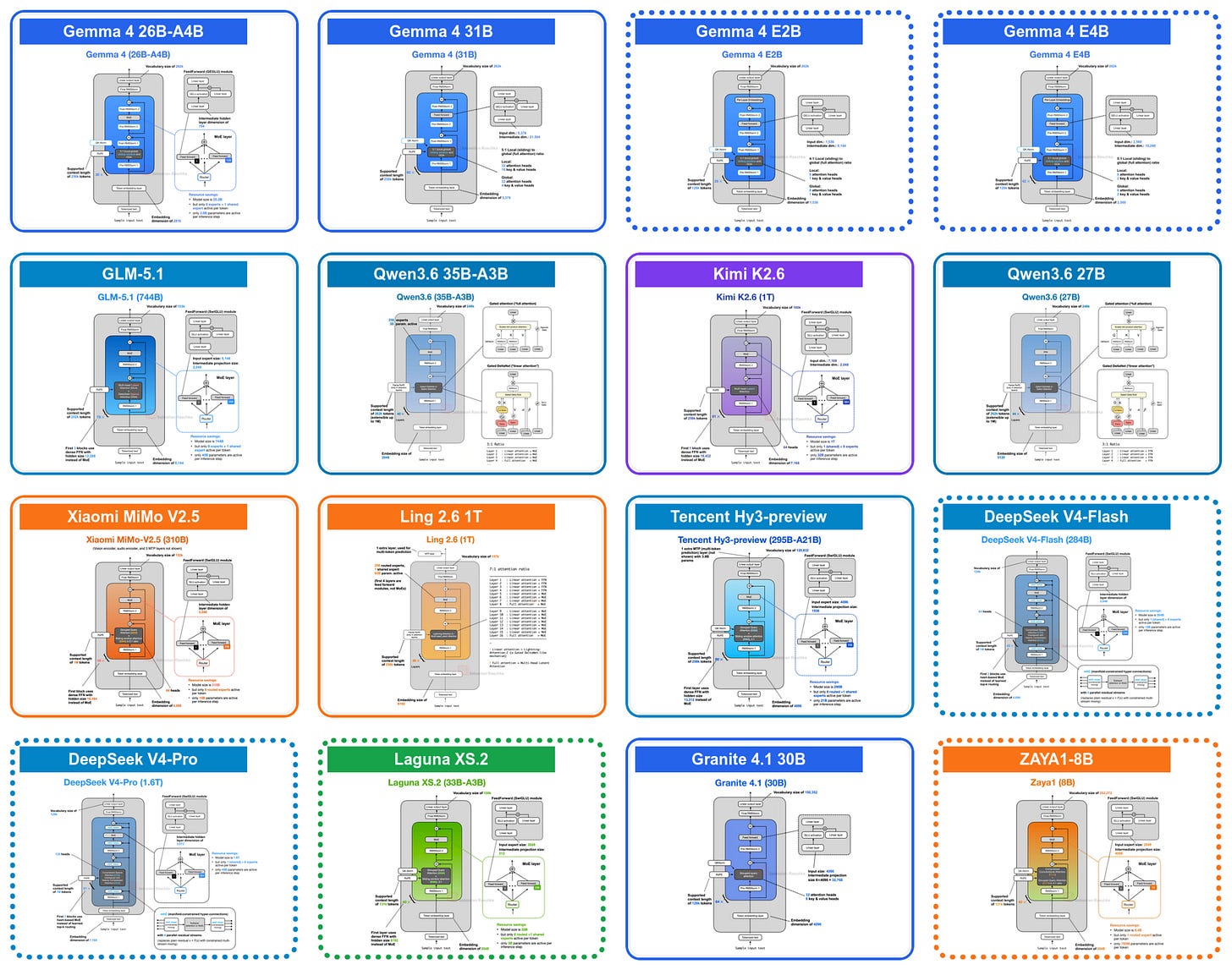
図 1. 直近の主要なオープンウェイトリリース(4 月から 5 月)における LLM アーキテクチャの描画。これらの画像や詳細は、私の LLM アーキテクチャギャラリーでご覧いただけます。すべてのモデルサイズが示されているわけではありません。Qwen3.6 では 27B および 35B-A3B バリアントが含まれており、ZAYA1 は 8B モデルで代表されています(ZAYA1-base および ZAYA1-reasoning-base は省略)。点線で囲まれたボックス内のアーキテクチャについては、本記事でより詳細に解説します。
なお、本記事はアーキテクチャ設計に関するものであるため、データセットの混合比率、トレーニングスケジュール、ポストトレーニングの詳細、RL(強化学習)レシピ、ベンチマーク表、製品比較については主に省略させていただきます。このように範囲を狭めたとしても、扱うべき内容は依然として多岐にわたります。いつも通り、本記事も予想以上に長くなってしまいましたので、トランスフォーマーブロック内部の変化、リジューアルストリーム(残差流)、KV キャッシュ、あるいはアテンション計算における変更点に焦点を絞って解説します。
また、私が取り上げるのは、興味深い(新規の)設計選択であり、かつ他でまだカバーしていないトピックのみです。このリストには以下が含まれます:
Gemma 4 における KV シェアリングと層ごとの埋め込み
ZAYA1 における圧縮畳み込みアテンション
Laguna XS.2 におけるアテンション予算管理
DeepSeek V4 における mHC および圧縮アテンション
過去のトピック
新しい部分に入る前に、参照する以前の 2 つの記事をご紹介します。1 つ目は、最近の MoE モデル、ルーティングされたエキスパート、アクティブパラメータ、モデルサイズの比較に関する広範なアーキテクチャ背景を扱っています。2 つ目は、以下で繰り返し登場するアテンションの背景をカバーしており、MHA、MQA、GQA、MLA、スライディングウィンドウアテンション、スパースアテンション、ハイブリッドアテンション設計が含まれます。
私はこれらの解説の一部を、LLM アーキテクチャギャラリー内の短く独立したチュートリアルページにもまとめました。例えば、読者は対応するモデルカードやコンセプトラベルからリンクされている GQA、MLA、スライディングウィンドウアテンション、DeepSeek スパースアテンション、MoE ルーティングなどの概念に関するコンパクトな解説を見つけることができます。
- KV テンソルを層間で再利用してキャッシュを縮小する(Gemma 4)
アーキテクチャの進展と微調整のこのツアーでは、Google が新しいオープンウェイトの Gemma 4 モデルスイートをリリースした 4 月初めに戻りましょう。これらは 3 つの主要なカテゴリに分かれています。
モバイルや小型のローカル(埋め込み)デバイス(いわゆる IoT)向けの Gemma 4 E2B および E4B モデル、
効率的なローカル推論に最適化された Gemma 4 26B ミクスチャー・オブ・エキスパート(MoE)モデル、
そして最大品質とより便利なトレーニング後処理(MoE は扱いが難しいため)のための Gemma 4 31B デンサーモデルです。
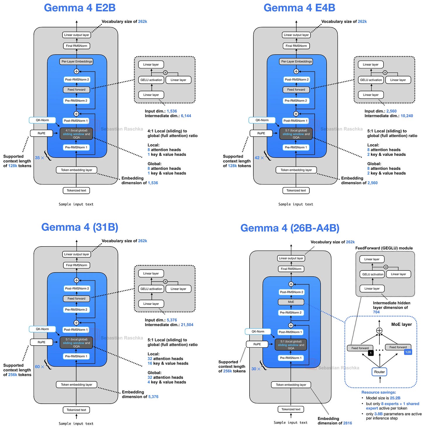
図 2: Gemma 4 のアーキテクチャ図。
E2B および E4B バリアントにおける最初の小さなアーキテクチャの改良点は、共有 KV キャッシュ(Key-Value Cache)方式を採用していることです。この方式では、後段のレイヤーが前段のレイヤーからのキー・バリュー状態を再利用し、長期コンテキストにおけるメモリ使用量と計算コストを削減します。
この KV 共有の概念は Gemma 4 が発明したわけではありません。例えば、Brandon らによる「Reducing Transformer Key-Value Cache Size with Cross-Layer Attention」(NeurIPS 2024)をご覧ください。しかし、私がこの概念が適用された例として最初に目にしたのは、まさにこの人気のあるアーキテクチャでした。(なお、クロスレイヤー・アテンションはクロス・アテンションとは混同しないでください。)
KV 共有についてさらに説明する前に、その動機について簡単に触れておきましょう。最近数ヶ月間、私が執筆し議論してきた通り、LLM(大規模言語モデル)アーキテクチャ設計における主要なテーマの一つが、KV キャッシュサイズの削減です。その背後にある動機は、必要なメモリ量を減らすことであり、これによりより長いコンテキストを扱えるようになります。これは特に、推論モデルやエージェントの時代において重要な意義を持ちます。KV キャッシングに関する詳細な背景については、私の「Understanding and Coding the KV Cache in LLMs from Scratch」の記事をご覧ください。
私が以前の記事「現代の LLM におけるアテンション変種への視覚的ガイド」で説明した人気のあるアテンション変種のほとんどは、KV キャッシュサイズを削減するために設計されています:
古典的な例(Gemma 4 もまだ使用しています)を挙げると:グループ化クエリアテンション(GQA: Grouped Query Attention)は、図に示すように、異なるクエリヘッド間でキー・バリュー(KV: Key-Value)ヘッドを共有することで KV キャッシュサイズを削減します。
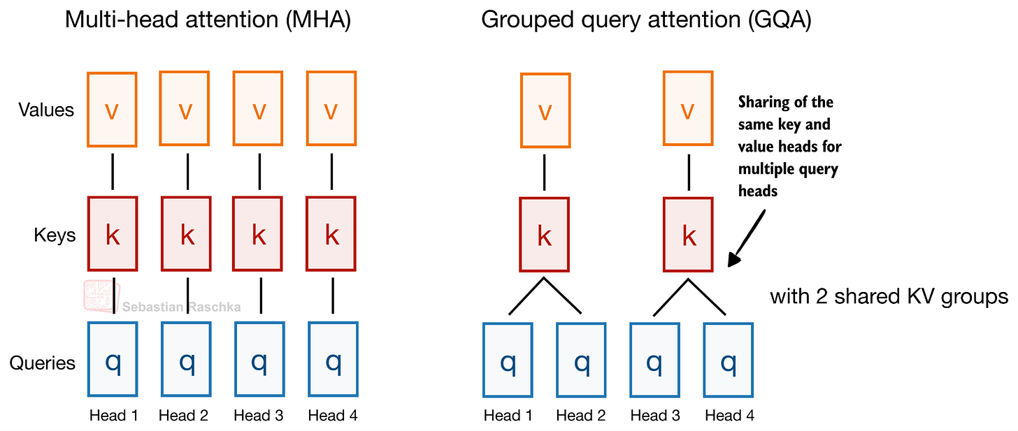
図 3: グループ化クエリアテンション(GQA)は、複数のクエリ(Q: Query)ヘッド間で同じキー(K: Key)およびバリュー(V: Value)ヘッドを共有します。
前述の通り、Gemma 4 は GQA を使用しています。しかし、GQA の一部としてクエリ間での KV 共有に加えて、Gemma 4 は各層のアテンションモジュールの一部として計算するのではなく、異なる層間で KV プロジェクションも共有します。この KV 共有方式はクロスレイヤーアテンションとも呼ばれ、以下の図に示されています。
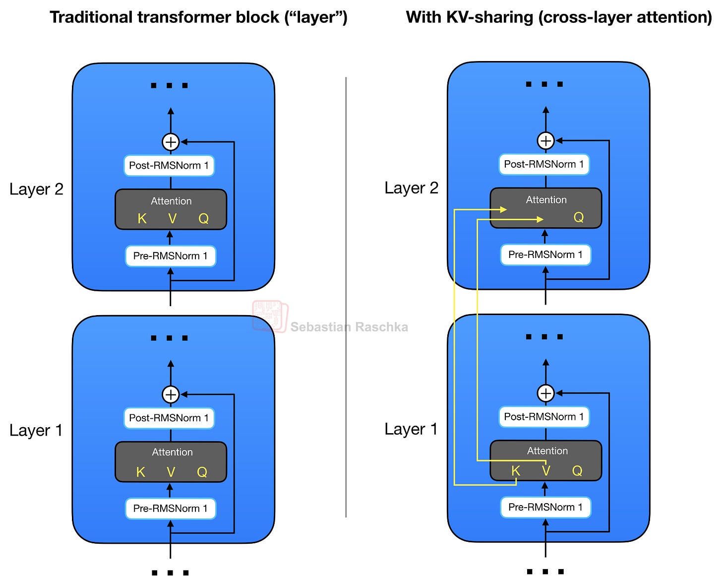
図 4:通常のトランスフォーマーブロックは、各アテンションモジュール内で独立した Q(クエリ)、K(キー)、V(バリュー)射影を計算します(左)。クロスレイヤーアテンション設計(右)では、複数の層にわたって同じ K と V の射影が共有されます。
図 2 のアーキテクチャ概要で簡潔に触れられている通り、Gemma 4 E2B は 4:1 のパターンで通常の GQA(Grouped Query Attention)とスライディングウィンドウアテンションを使用しています。(より正確には、Gemma 4 E2B は MQA(Multi-Query Attention)を採用しており、これは GQA の一 K 一 V ヘッドという特殊ケースです。)
GQA(または MQA)の場合の KV 共有は以下の通り機能します。後続の層は独自のキーおよびバリュー射影を計算するのではなく、同じアテンションタイプを持つ直前の非共有層からの KV テンソルを再利用します。言い換えれば、スライディングウィンドウ層は以前のスライディングウィンドウ層と KV を共有し、フルアテンション層は以前のフルアテンション層と KV を共有します。各層は依然として独自のクエリ射影を計算するため、それぞれの層が独自のアテンションパターンを形成できますが、高コストでメモリ消費の大きい KV キャッシュ(Key-Value Cache)は複数の層にわたって再利用されます。
例えば、Gemma 4 E2B は 35 個のトランスフォーマー層を持ちますが、KV 射影を独自に計算するのは最初の 15 層のみで、残りの最終 20 層は同じアテンションタイプを持つ直前の非共有層からの KV テンソルを再利用します。同様に、Gemma 4 E4B は 42 層を持ち、そのうち 24 層が独自の KV を計算し、最後の 18 層でそれらを共有しています。
実際にどれほど節約できるのでしょうか?層間で KV の約半分を共有するため、KV キャッシュのサイズは概ね半分に削減されます。最小サイズの E2B モデルでは、128K という長いコンテキストにおいて bfloat16 精度で約 2.7 GB の節約になります(以下参照)。(E4B バリアントの場合、128K で約 6 GB 節約されます。)
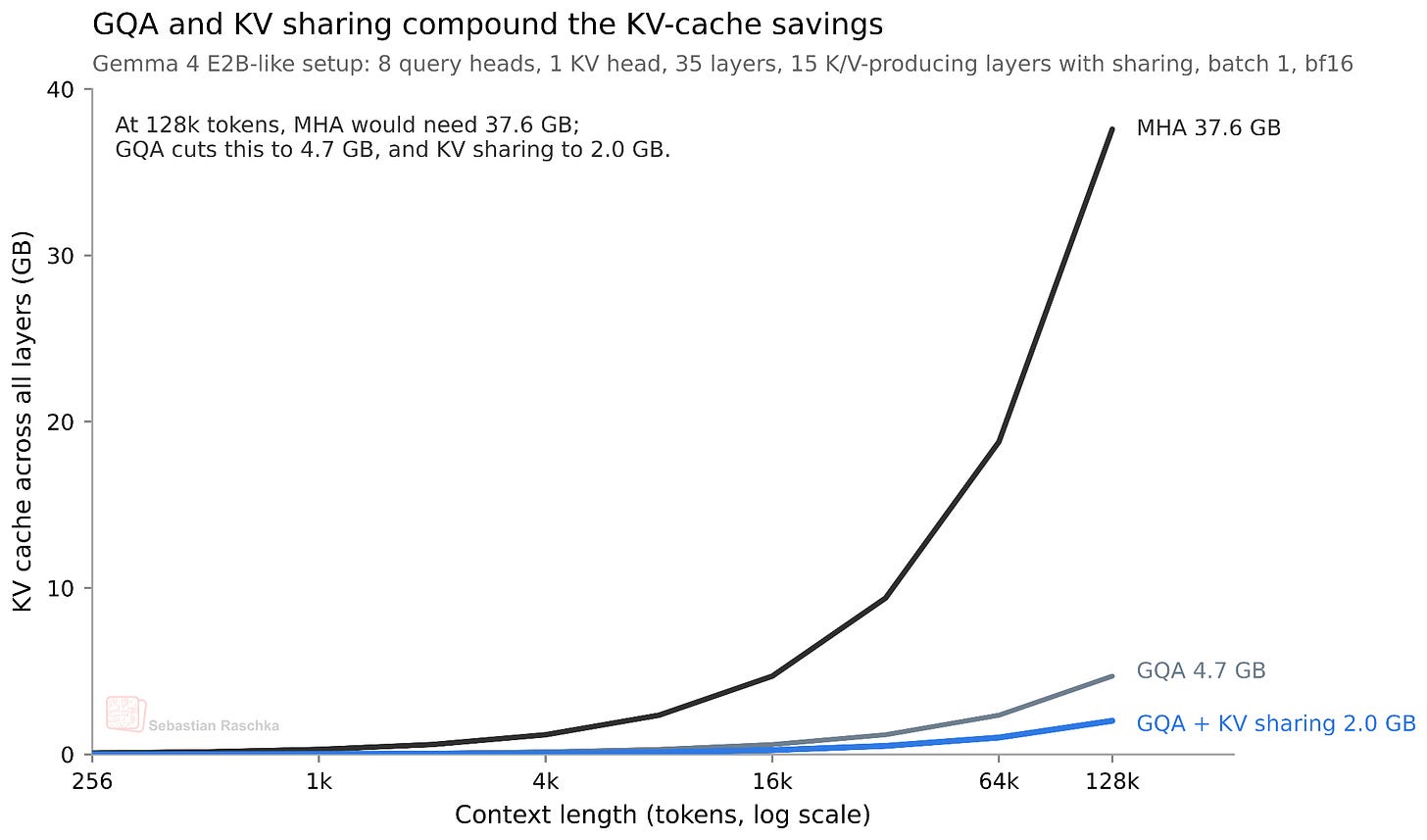
図 5: Gemma 4 E2B に似た設定における GQA(Grouped Query Attention)と層間 KV 共有による KV キャッシュのメモリ節約効果。簡略化のため、スライディングウィンドウアテンションからの追加的な節約効果は示していません。
KV 共有の欠点は、もちろんそれが「近似」であることです。より正確に言えば、モデルの容量が低下します。しかし、層間アテンションに関する論文によると、その影響は最小限です(テストされた小規模モデルにおいては)。
- 層別埋め込みと「実効的」サイズ (Gemma 4 E2B/E4B)
Gemma 4 の E2B および E4B バリアントには、KV 共有スキームとは別に、効率性を重視したもう一つの設計選択である「層別埋め込み(Per-Layer Embeddings: PLE)」が含まれています。
KV 共有は KV キャッシュを削減するものですが、PLE はパラメータ効率に関するものです。これにより、小規模な Gemma 4 モデルは、同じ総パラメータ数を持つ密結合モデルほどトランスフォーマースタックのコストを増やすことなく、より多くのトークン固有の情報を活用できるようになります。
例えば、Gemma 4 E2B および E4B における「E」とは「effective(有効)」を意味します。具体的には、Gemma 4 E2B は有効パラメータ数が 23 億と記載されていますが、埋め込み層のパラメータを含めると 51 億となります。(同様に、Gemma 4 E4B は有効パラメータ数 45 億、埋め込み層を含むと 80 億と記載されています。)
要するに、「E」モデルでは、主要なトランスフォーマースタックの計算量は小さい方の数値に近いですが、大きい方の数値には追加の埋め込みテーブル層が含まれています。(埋め込み層がどのように機能するかについては、私の「Embedding Layers と Linear Layers の違いを理解する」というコードノートブックをご覧ください。)
概念的に、新しい PLE パスは以下のようになります。
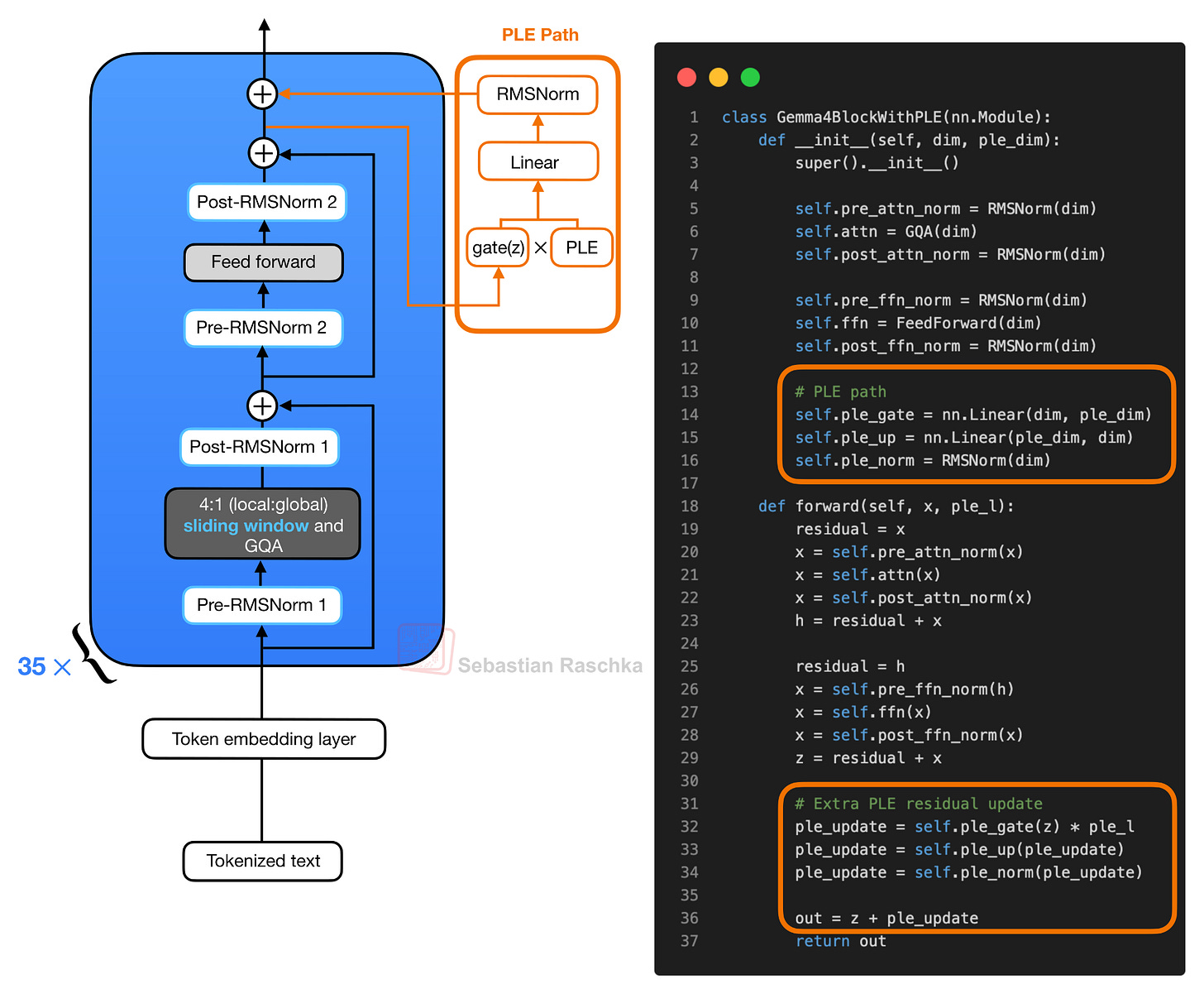
図 6:PLE の残差パスを備えた簡略化された Gemma 4 ブロック。通常のブロックはまずアテンションとフィードフォワードの残差更新を計算します。得られた隠れ状態が層固有の PLE ベクトルをゲート制御し、投影された PLE 更新はブロックの最後に追加の残差更新として加算されます。
PLE ベクトル自体は、反復するトランスフォーマーブロックの外側で用意されます。簡略化された形式では、PLE 構築には 2 つの入力があります。第一に、トークン ID は層ごとの埋め込み検索を経由します。第二に、通常のトークン埋め込みは、同じパッキングされた PLE 空間へ線形射影されます。これら 2 つの要素を加算し、スケーリングした上で、層ごとに 1 スライスずつ持つテンソルへと再整形されます。各ブロックがそれぞれ独自のスライスを受け取る点に注意してください。
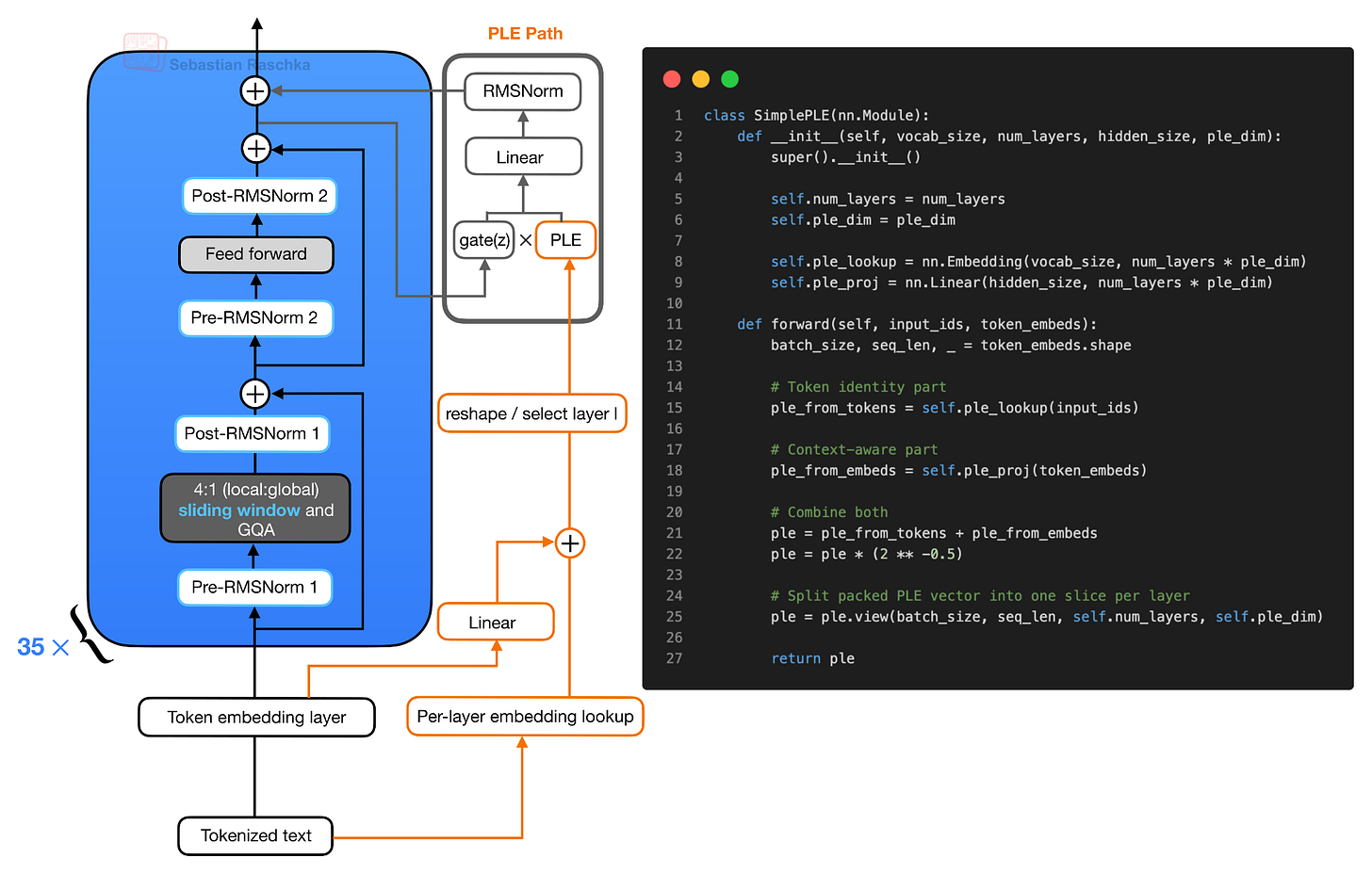
図 7: 簡略化された PLE 構築。トークン ID は層ごとの埋め込み検索を提供し、通常のトークン埋め込みは同じ空間へ射影されます。これら 2 つの寄与が結合され再整形されることで、各トランスフォーマーブロックは独自の層固有の PLE スライスを受け取ります。
重要な詳細は、PLE が各トランスフォーマーブロックに通常のトークン埋め込み層の完全な独立コピーを与えない点です。代わりに、層ごとの埋め込み検索は一度計算されるだけです。前述した通り、その後、各層には小さなトークン固有の埋め込みスライスが与えられます(「再整形 / 層 l の選択」経由)。
したがって、各入力トークンに対して、Gemma 4 はデコーダー層ごとに 1 つの小さなベクトルを含むパッキングされた PLE テンソルを用意します。その後、順伝播(フォワードパス)において、層 l は自身のスライスのみを受け取ります(図 6 の Gemma4WithPLEBlock における ple_l)。
トランスフォーマーブロック内部では、通常の注意機構とフィードフォワード分岐が通常通り動作します。まず、ブロックは注意の残差更新を計算し、次にフィードフォワードの残差更新を計算します。2 回目の残差加算の後、図 6 の疑似コードで z と表記した結果の隠れ状態が、層固有の PLE ベクトルをゲート制御するために使用されます。ゲート制御された PLE ベクトルはモデルの隠れサイズに投影され、正規化された後、追加の残差更新として加算されます。
したがって、有用な心的モデルとしては、トランスフォーマーブロックには依然として主要な注意機構とフィードフォワード経路が存在するが、Gemma 4 ではフィードフォワード分岐の後に小さな層固有トークンベクトルが追加されるというものです。これは埋め込みパラメータと小規模な投影を通じて表現能力を増加させます。これにより計算オーバーヘッドが増加しますが、トランスフォーマースタック全体をより大きなパラメータ数にスケールさせるコストを回避できます。
ではなぜ PLE(Per-Layer Embedding)なのでしょうか?より単純な代替案は、層数を減らしたり、隠れ状態の幅を狭くしたり、フィードフォワードネットワークを小さくしたりして、密結合モデルを小型化することです。これによりメモリ使用量とレイテンシが削減されますが、主要な計算を行うモデル部分からの容量も失われます。
PLE の設計では、高価なトランスフォーマーブロックをより小さな「実効」サイズに近い状態に保ちつつ、追加の容量は層ごとの埋め込みテーブルに格納します。これらは、主にキャッシュ可能なルックアップ形式のパラメータであるため、さらに多くの注意機構や FFN(Feed-Forward Network)重みを追加するよりもはるかに安価に利用できます。
また、この設計が効果的かつ価値のある選択であると Google の言葉を信じる必要があります。この E2B 設計が通常の Gemma 4 2.3B モデルや通常の Gemma 4 5.1B モデルと比較してどうなるかを示す比較研究が行われると興味深いでしょう。
また、原則として PLE は小規模モデルに固有の制限があるわけではありません。大規模モデルに対しても層ごとの埋め込みスライスを追加することは可能です。しかし、大規模モデルはすでに十分な容量を持っており、これらの追加埋め込みがそれほど役立たない可能性があります。さらに、大規模モデルでは、計算負荷を小さく保ちながら容量を増やすためのトリックとして、すでに MoE(Mixture of Experts)設計を採用しています。
ちなみに、比較的シンプルで読みやすいコード実装に興味がある場合は、Gemma 4 の E2B および E4B モデルをゼロから実装したものをこちらで公開しています。
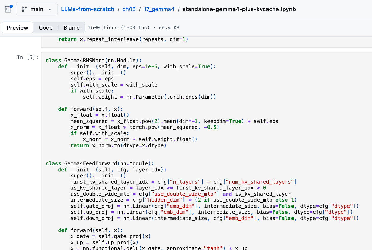
図 8: ゼロから実装した私の Gemma 4 のスナップショット。
- レイヤー別アテンション予算管理 (Laguna XS.2)
Laguna は、コーディングアプリケーション向けの LLM 訓練に注力するヨーロッパ拠点の企業である Poolside が初めて公開重み(オープンウェイト)モデルとしてリリースしたものです。私の元同僚数名が近年 Poolside に合流しており、彼らは才能あふれる素晴らしいチームを築いています。他の企業も自社のモデルの一部をオープンウェイト版としてリリースしているのを目にするのは嬉しいことです。
さて、以下に示す Laguna XS.2 アーキテクチャは、一見すると非常に標準的なものに見えます。しかし、私がここ (/try to cram into there) で示さなかった(あるいは詰め込もうとした)重要な詳細として、「レイヤーごとのアテンション予算配分」という概念があります。
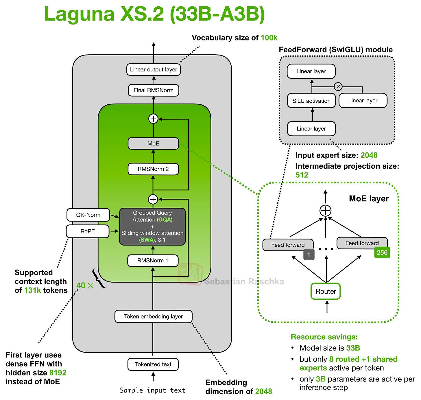
図 9: Poolside の Laguna XS.2 アーキテクチャ。
ここで提案されているアテンション予算配分の考え方の一部は、すべてのトランスフォーマー層に同じ完全なアテンション予算を与えるのではなく、Laguna XS.2 では層ごとにアテンションコストを変化させるという点にあります。このアーキテクチャには合計 40 層があり、そのうち 30 層がスライディングウィンドウ・アテンション(sliding-window attention)層で、10 層がグローバル/フル・アテンション(global/full attention)層です。通常通り、スライディングウィンドウ層はローカルなウィンドウ内(ここでは 512 トークン)のみを参照するため、KV キャッシュとアテンション計算のコストを抑えることができます。一方、グローバル層はコストがかかりますが、コンテキストウィンドウ内のすべての情報にアクセスする能力を保持します。
このスライディングウィンドウ・アテンションとグローバル/フル・アテンションを組み合わせたパターンは Laguna XS.2 固有のものではなく、Gemma 4 を含む多くの他のアーキテクチャでも採用されています。
しかし、新しい点はレイヤーごとのクエリヘッド数の使用です。例えば、Hugging Face のモデルハブの config.json には num_attention_heads_per_layer という設定が含まれており、これにより各層が異なる数のクエリヘッドを持つことが可能になりつつも、KV キャッシュの形状は互換性を保つことができます。
図 10: Laguna における層ごとのクエリ・ヘッド予算配分。フルアテンション層では KV ヘッドあたり 6 クエリ・ヘッドを使用し、スライディングウィンドウアテンション層では KV ヘッドあたり 8 クエリ・ヘッドを使用します。
Laguna XS.2 は、スライディングウィンドウ層により多くのクエリ・ヘッドを割り当て、グローバル層にはより少ないクエリ・ヘッドを割り当てる一方、KV ヘッドは固定で 8 に保つという、この層ごとのクエリ・ヘッド予算配分の最も顕著な最近の事例の一つです。これが設定における実際の層別ヘッド予算配分です。
Laguna XS.2 は、本番環境向けオープンモデルにおけるこの層ごとのクエリ・ヘッド予算配分の代表的な例の一つですが、層ごとにモデル容量を変化させるというより広範なアイデアは、少なくとも Apple の 2024 年発表の OpenELM にまで遡ります。
では、このような設計の目的は何でしょうか?KV 共有と同様に、その目的は、すべての層に同じ予算を与えるのではなく、アテンション容量を最も有用な場所に投資することです。具体的には、フルアテンション層は文脈全体を参照するため高コストとなるため、Laguna はスライディングウィンドウアテンションモジュールと比較して、これらに割り当てるクエリ・ヘッド数を減らしています。
(なお、もう一つの小さな実装詳細として、Laguna はヘッドごとのアテンション出力ゲートも適用しています。これは Qwen3-Next や他モデルとある程度類似しており、以前の記事で既に扱っているためここでは省略します。)
- 圧縮畳み込みアテンション (ZAYA1-8B)
ラガナと同様に、ZAYA1-8B はオープンウェイト市場における新たなプレイヤーです。これは Zyphra によって開発されましたが、リリースに関する興味深い点の一つは、このモデルがより一般的な NVIDIA GPU(または Google TPU)ではなく、AMD GPU でトレーニングされたことです。
しかし、主なアーキテクチャの詳細は、グループ化クエリアテンション(Grouped-Query Attention: GQA)と共に使用される圧縮畳み込みアテンション(Compressed Convolutional Attention: CCA)です。MLA スタイルの設計が主に潜在表現をコンパクトな KV キャッシュ形式として使用するのに対し、CCA は圧縮された潜在空間内で直接アテンション演算を実行します。これについては後ほど詳しく説明します。
(補足:ZAYA1-8B の config.json には、従来の 40 ブロックではなく、80 の交互層エントリが記載されています。これらのエントリは CCA/GQA アテンションと MoE フィードフォワード層の間で交互に配置されます。しかし、アーキテクチャ図においては、これを概念上等価な「アテンション+MoE ペアの 40 回の繰り返し」として可視化するのがより便利です。)
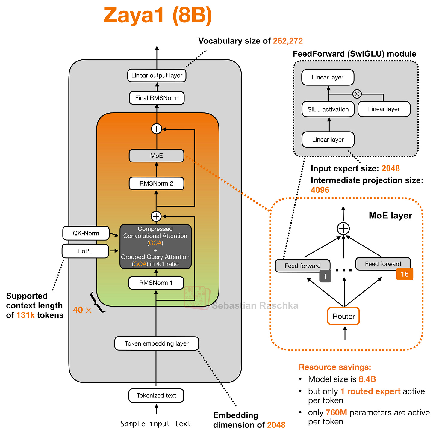
図 11: 圧縮畳み込みアテンションを備えたトランスフォーマーブロックを持つ Zaya1 (8B)。
上記の図で示唆されている通り、ZAYA1-8B は Compressed Convolutional Attention(CCA)と 4:1 の GQA レイアウトを組み合わせて使用しています。重要な点は、そのアテンションブロックが標準的なスライディングウィンドウアテンションブロックではなく、CCA を中心に構築されていることです。
圧縮畳み込みアテンションとは何か?
CCA は DeepSeek のモデルにおけるマルチヘッド潜在アテンション(MLA)と精神的に類似していると言えます。両者ともアテンションブロック内に圧縮された潜在表現を導入しているためです。ただし、その潜在空間の使い方は異なります。MLA は主に KV キャッシュを削減するためにこの潜在表現を利用します。MLA では KV テンソルがコンパクトに保存され、実際の計算のためにアテンションヘッド空間へ投影されます。
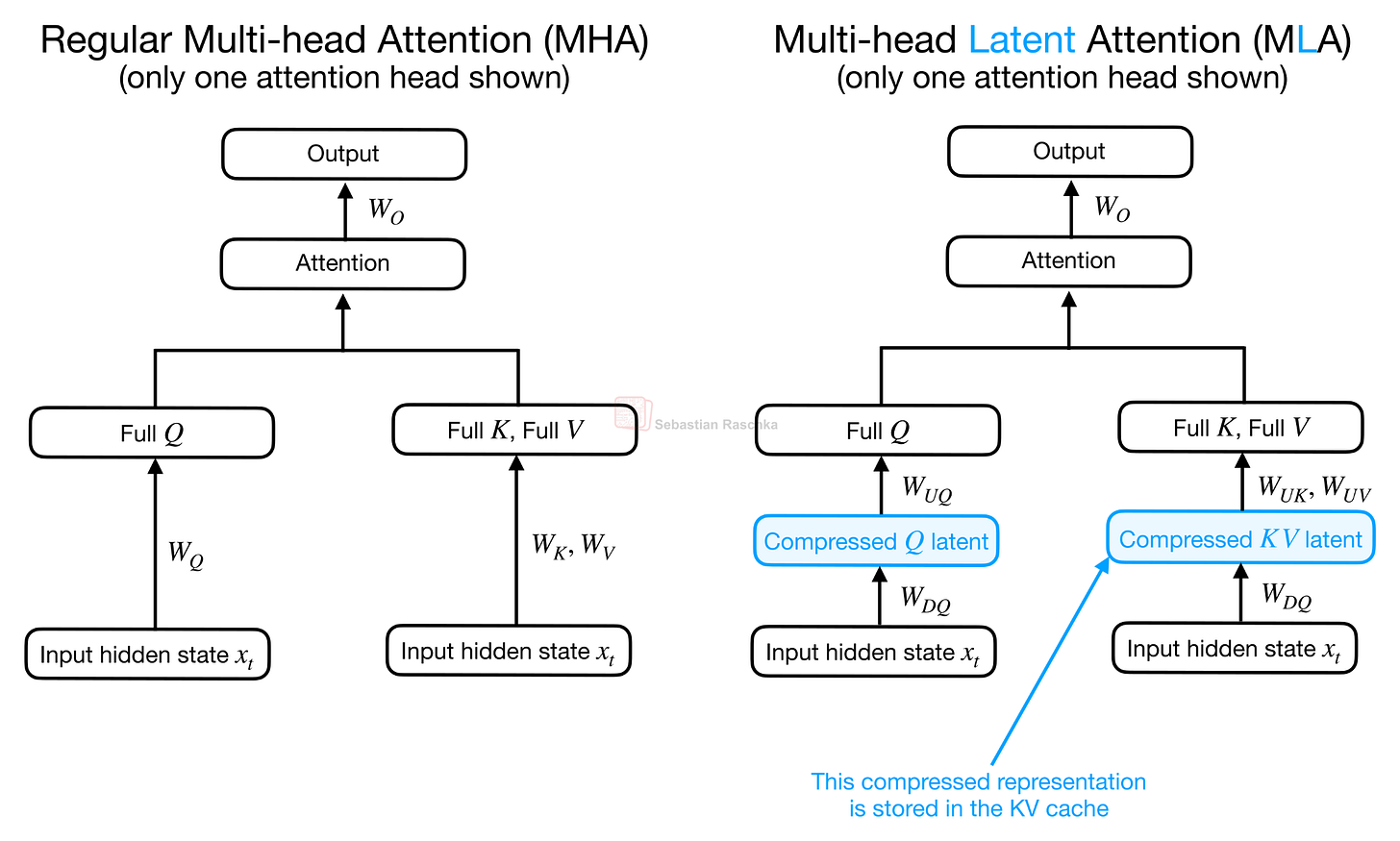
図 12: 並列した通常のマルチヘッドアテンション(MHA)とマルチヘッド潜在(MLA)アテンション。
CCA は Q、K、V を圧縮し、穿孔
原文を表示
After a short family break, I am excited to be back and catching up on a busy few weeks of open-weight LLM releases. The thing that stood out to me is how much newer architectures are focused on long-context efficiency.
As reasoning models and agent workflows keep more tokens around (for longer), KV-cache size, memory traffic, and attention cost quickly become the main constraints, and LLM developers are adding a growing number of architecture tricks to reduce those costs.
The main examples I want to look at are KV sharing and per-layer embeddings in Gemma 4, layer-wise attention budgeting in Laguna XS.2, compressed convolutional attention in ZAYA1-8B, and mHC plus compressed attention in DeepSeek V4.
Most of these changes look like small tweaks in my architecture diagrams, but some of them are quite intricate design changes that are worth a more detailed discussion.
Figure 1. LLM architecture drawings of recent, major open-weight releases (April to May). You can find the images, and more details, in my LLM architecture gallery. Not all model sizes are shown; Qwen3.6 includes the 27B and 35B-A3B variants, and ZAYA1 is represented by the 8B model (omitting ZAYA1-base and ZAYA1-reasoning-base). The architectures in the dotted boxes are covered in more detail in this article.
Note that this article is about architecture designs, so I will mostly skip dataset mixtures, training schedules, post-training details, RL recipes, benchmark tables, and product comparisons. Even with that narrower scope, there is a lot to cover. And, like always, the article turned out longer than I expected, so I will keep the focus on what changes inside the transformer block, residual stream, KV cache, or attention computation.
Please also note that I am only covering those topics that are interesting (new) design choices and that I haven’t covered elsewhere, yet. This list includes:
KV sharing and per-layer embeddings in Gemma 4
Compressed convolutional attention in ZAYA1
Attention budgeting in Laguna XS.2
mHC and compressed attention in DeepSeek V4
Previous Topics
Before getting into the new parts, here are the two previous articles I will refer back to. The first one gives a broader architecture background on recent MoE models, routed experts, active parameters, and model-size comparisons. The second one covers the attention background that comes up repeatedly below, including MHA, MQA, GQA, MLA, sliding-window attention, sparse attention, and hybrid attention designs.
I also turned several of these explanations into short, standalone tutorial pages in the LLM Architecture Gallery. For example, readers can find compact explainers for GQA, MLA, sliding-window attention, DeepSeek Sparse Attention, MoE routing, and other concepts linked from the corresponding model cards and concept labels.
- Reusing KV Tensors Across Layers to Shrink the Cache (Gemma 4)
For this tour of architecture advances and tweaks, we will go back to the beginning of April when Google released their new open-weight Gemma 4 suite of models. They come in 3 broad categories:
the Gemma 4 E2B and E4B models for mobile and small, local (embedded) devices (aka IoT),
the Gemma 4 26B mixture-of-experts (MoE) model, optimized for efficient local inference,
and the Gemma 4 31B dense model, for maximum quality and more convenient post-training (since MoEs are trickier to work with)
Figure 2: Gemma 4 architecture drawings.
The first small architecture tweak in the E2B and E4B variants is that they adopt a shared KV cache scheme, where later layers reuse key-value states from earlier layers to reduce long-context memory and compute.
This KV-sharing was not invented by Gemma 4. For instance, see Brandon et al., “Reducing Transformer Key-Value Cache Size with Cross-Layer Attention” (NeurIPS 2024). But it’s the first popular architecture where I saw this concept applied. (Cross-layer attention is not to be confused with cross-attention.)
Before explaining KV-sharing further, let’s briefly talk about the motivation. As I wrote and talked about in recent months, one of the main recent themes in LLM architecture design is KV cache size reduction. In turn, the motivation behind KV cache size reduction is to reduce the required memory, which allows us to work with longer contexts, which is especially relevant in the age of reasoning models and agents. For more background on KV caching, see my “Understanding and Coding the KV Cache in LLMs from Scratch” article:
Practically all of the popular attention variants I described in my previous A Visual Guide to Attention Variants in Modern LLMs article are designed to reduce the KV cache size:
To pick a classic example (that Gemma 4 still uses): Grouped Query Attention (GQA) already shares key-value (KV) heads across different query heads to reduce the KV cache size, as illustrated in the figure below.
Figure 3: Grouped Query Attention (GQA) shares the same key (K) and value (V) heads among multiple query (Q) heads.
As mentioned before, Gemma 4 uses GQA. However, in addition to the KV sharing among queries as part of GQA, Gemma 4 also shares KV projections across different layers instead of computing it as part of the attention module in each layer. This KV-sharing scheme, also called cross-layer attention, is illustrated in the figure below.
Figure 4: Regular transformer blocks compute separate Q, K, and V projections in each attention module (left). Cross-layer attention designs (right) share the same K and V projections across multiple layers.
As briefly hinted at in the architecture overview in Figure 2, Gemma 4 E2B uses regular GQA and sliding window attention in a 4:1 pattern. (More precisely, Gemma 4 E2B uses MQA, which is the one-KV-head special case of GQA).
In the case of GQA (or MQA), the KV-sharing works like this. Later layers no longer compute their own key and value projections but reuse the KV tensors from the most recent earlier non-shared layer of the same attention type. In other words, sliding-window layers share KV with a previous sliding-window layer. Full-attention layers share KV with a previous full-attention layer. The layers still compute their own query projections, so each layer can form its own attention pattern, but the expensive and memory-heavy KV cache is reused across several layers.
For example, Gemma 4 E2B has 35 transformer layers, but only the first 15 compute their own KV projections; the final 20 layers reuse KV tensors from the most recent earlier non-shared layer of the same attention type. Similarly, Gemma 4 E4B has 42 layers, with 24 layers computing their own KV and the final 18 layers sharing them.
How much does this actually save? Since we share roughly half of the KVs across layers, we save approximately half of the KV cache size. For the smallest E2B model, this results in a 2.7 GB saving (at bfloat16 precision) in long 128K contexts, as shown below. (For the E4B variant, this saves about 6 GB at 128K.)
Figure 5: KV cache memory savings from GQA and cross-layer KV sharing in a Gemma 4 E2B-like setup. For simplicity, additional savings from sliding window attention are not shown.
The downside of KV-sharing is, of course, that it’s an “approximation” of the real thing. Or, more precisely, it reduces model capacity. However, according to the cross-layer attention paper, the impact can be minimal (for small models that were tested).
- Per-Layer Embeddings and “Effective” Size (Gemma 4 E2B/E4B)
The Gemma 4 E2B and E4B variants include a second efficiency-oriented design choice called per-layer embeddings (PLE). This is separate from the KV-sharing scheme above.
KV sharing reduces the KV cache. PLE is instead about parameter efficiency, where it lets the small Gemma 4 models use more token-specific information without making the main transformer stack as expensive as a dense model with the same total parameter count.
For instance, the “E” in Gemma 4 E2B and E4B stands for “effective”. Concretely, Gemma 4 E2B is listed as 2.3B effective parameters, or 5.1B parameters when the embeddings are counted. (Similarly, Gemma 4 E4B is listed as 4.5B effective parameters, or 8B parameters with embeddings).
In short, in the “E” models, the main transformer-stack compute is closer to the smaller number, while the larger number includes the additional embedding-table layers. (For an illustration of how embedding layers work, see my “Understanding the Difference Between Embedding Layers and Linear Layers” code notebook.)
Conceptually, the new PLE path looks like this:
Figure 6: Simplified Gemma 4 block with the PLE residual path. The normal block first computes the attention and feed-forward residual updates. The resulting hidden state gates the layer-specific PLE vector, and the projected PLE update is added as an extra residual update at the end of the block.
The PLE vectors themselves are prepared outside the repeated transformer blocks. In simplified form, there are two inputs to the PLE construction. First, the token IDs go through a per-layer embedding lookup. Second, the normal token embeddings go through a linear projection into the same packed PLE space. These two pieces are added, scaled, and reshaped into a tensor with one slice per layer. Note that each block then receives its own slice.
Figure 7: Simplified PLE construction. The token IDs provide a per-layer embedding lookup, while the normal token embeddings are projected into the same space. The two contributions are combined and reshaped so that each transformer block receives its own layer-specific PLE slice.
The important detail is that PLE does not give each transformer block a full independent copy of the normal token embedding layer. Instead, the per-layer embedding lookup is computed once. Then, as mentioned before, it gives each layer a small token-specific embedding slice (via “reshape / select layer l”.
So, for each input token, Gemma 4 prepares a packed PLE tensor that contains one small vector per decoder layer. Then, during the forward pass, layer l receives only its own slice (ple_l in the Gemma4WithPLEBlock in figure 6).
Inside the transformer block, the regular attention and feed-forward branches run as usual. First, the block computes the attention residual update. Then it computes the feed-forward residual update. After that second residual add, the resulting hidden state, which I denoted as z in the pseudocode in figure 6, is used to gate the layer-specific PLE vector. The gated PLE vector is projected back to the model hidden size, normalized, and added as one extra residual update.
So the useful mental model is that the transformer block still has the same main attention and feed-forward path, but Gemma 4 adds a small layer-specific token vector after the feed-forward branch. This increases representational capacity through embedding parameters and small projections. This adds computational overhead but avoids the cost of scaling the entire transformer stack to the larger parameter count.
But why PLEs? The simpler alternative would be to make the dense model smaller, using fewer layers, narrower hidden states, or smaller feed-forward networks. That would reduce memory and latency, but it also removes capacity from the parts of the model that do the main computation.
The PLE design keeps the expensive transformer blocks closer to the smaller “effective” size, while storing additional capacity in per-layer embedding tables. These are much cheaper to use than adding more attention or FFN weights, since they are mainly lookup-style parameters that can be cached.
Also, we have to take Google’s word here that this is an effective and worthwhile design choice. It would be interesting to see some comparison studies to see how this E2B design compares to a regular Gemma 4 2.3B model and a regular Gemma 4 5.1B model.
Also, in principle, PLE is not inherently limited to small models. We could attach per-layer embedding slices to larger models, too. However, larger models already have sufficient capacity where these extra embeddings may not help that much. Also, for larger models, we already use MoE designs as a trick to increase capacity while keeping the compute footprint smaller.
By the way, if you are interested in a relatively simple and readable code implementation, I implemented the Gemma 4 E2B and E4B models from scratch here.
Figure 8: Snapshot of my Gemma 4 from-scratch implementation.
- Layer-Wise Attention Budgeting (Laguna XS.2)
Laguna is the first open-weight model by Poolside, a Europe-based company focused on training LLMs for coding applications. Several of my former colleagues joined Poolside in recent years, and they have a great team with lots of talent. It’s just nice to see more companies also releasing some of their models as open-weight variants.
Anyways, the Laguna XS.2 architecture depicted below looks very standard at first glance. However, one detail that I didn’t show (/try to cram into there) is a concept we can refer to as “Layer-wise attention budgeting”.
Figure 9: Poolside’s Laguna XS.2 architecture.
Part of the idea behind the attention budgeting here is that instead of giving every transformer layer the same full attention budget, Laguna XS.2 varies the attention cost by layer. It has 40 layers total, with 30 sliding-window attention layers and 10 global/full attention layers. As usual, the sliding-window layers only attend over a local window (here: 512 tokens), which keeps the KV cache and attention computation cheaper. The global layers are more expensive but preserve the ability to access all information in the context window.
This mixed sliding-window + global/full attention pattern is not unique to Laguna XS.2 and is used by many other architectures (including Gemma 4).
But what’s new is the use of per-layer query-head counts. For instance, the Hugging Face model hub config.json includes a num_attention_heads_per_layer setting, so layers can have different numbers of query heads while keeping the KV cache shape compatible.
Figure 10: Per-layer query-head budgeting in Laguna, where full attention layers use 6 query heads per KV head, and sliding window attention layers use 8 query heads per KV head.
So Laguna XS.2 gives more query heads to sliding-window layers and fewer query heads to global layers, while keeping the KV heads fixed at 8. That is the actual layer-wise head budgeting in the config.
Laguna XS.2 is one of the most prominent recent examples of this per-layer query-head budgeting in a production-style open model. But the broader idea of varying model capacity by layer goes back to (at least) Apple’s 2024 OpenELM.
And again, what’s the point of such a design? Similar to KV-sharing, the point is to spend attention capacity where it is most useful, instead of giving every layer the same budget. Specifically, full-attention layers are expensive because they look across the whole context, so Laguna gives them fewer query heads compared to sliding window attention modules.
(Besides, another smaller implementation detail is that Laguna also applies per-head attention-output gating; this is somewhat similar to Qwen3-Next and others, which I also omit here since I covered it in earlier articles.)
- Compressed Convolutional Attention (ZAYA1-8B)
Similar to Laguna, ZAYA1-8B is another new player on the open-weight market. It is developed by Zyphra, and one of the interesting details around the release is that the model was trained on AMD GPUs rather than the more common NVIDIA GPU (or Google TPU) setup.
The main architecture detail, though, is Compressed Convolutional Attention (CCA), used together with grouped-query attention. Unlike MLA-style designs that mainly use a latent representation as a compact KV cache format, CCA performs the attention operation directly in the compressed latent space, but more on that later.
(Sidenote: the ZAYA1-8B config.json lists 80 alternating layer entries rather than 40 conventional transformer blocks. These entries alternate between CCA/GQA attention and MoE feed-forward layers. But for the architecture figure, it is more convenient to visualize this as 40 repeated attention + MoE pairs, which is conceptually equivalent.)
Figure 11: Zaya1 (8B) with transformer blocks featuring compressed convolutional attention.
As hinted at in the figure above, ZAYA1-8B uses Compressed Convolutional Attention (CCA) together with a 4:1 GQA layout. The key point is that its attention block is built around CCA rather than a standard sliding-window attention block.
What is Compressed Convolutional Attention?
I would say CCA is related in spirit to Multi-head Latent Attention (MLA) in DeepSeek’s models, since both introduce a compressed latent representation into the attention block. However, they use that latent space differently. MLA mainly uses the latent representation to reduce the KV cache. In MLA, the KV tensors are stored compactly and then projected into the attention-head space for the actual attention computation.
Figure 12: Regular Multi-head Attention (MHA) and Multi-head Latent (MLA) attention side by side.
CCA compresses Q, K, and V and perfor
関連記事
今日のまとめ
AI日報で今日の重要ニュースをまとめ読み