SmithDB の全文検索用逆インデックス構築の仕組み
LangChain チームは、SmithDB における高速な全文検索機能の実現のために、カスタム設計された逆インデックスのアーキテクチャと実装プロセスを詳細に解説している。
キーポイント
逆インデックスの設計思想
大規模テキストデータに対する高速検索を実現するため、従来の汎用データベースではなく、LLM アプリケーションのユースケースに特化した独自の逆インデックス構造を採用した。
実装プロセスと最適化
インデックス構築時のメモリ効率や、検索クエリ処理におけるレイテンシ低減のために、データ構造の細部まで徹底的に最適化した実装が行われた。
SmithDB への統合と効果
この技術的改善により、LangChain アプリケーション内で複雑な全文検索タスクをネイティブかつ高速に実行可能となり、RAG パフォーマンスが向上した。
影響分析・編集コメントを表示
影響分析
この記事は、単なる機能追加ではなく、LLM アプリケーションの基盤となるデータベース設計における「検索」の重要性と、それを支える技術的アプローチの深さを示している。LangChain のような主要フレームワークが自社のインフラに深く関与し、最適化を行う姿勢は、RAG システムのパフォーマンス限界を押し上げる重要な指針となり得る。
編集コメント
LangChain が自社のデータベース製品にまで手を伸ばし、検索性能の根幹を最適化している点は、フレームワークとインフラの境界が曖昧になる現代の AI エコシステムを象徴しています。
SmithDB における全文検索:逆インデックスの構築と照会(第 2 回)
概要
SmithDB で全文検索をサポートする方法について、以前のブログ記事 earlier blog post では、オブジェクトストレージをバックエンドとする逆インデックスの実装設計について解説しました。今回のブログ記事では、SmithDB においてこのインデックスをどのように構築し、コンパクション(圧縮統合)を行い、照会するかについて取り上げます。
逆インデックスの構築とマージ
インデックスの構築は、データ取り込み時に並行して行われます。新しいランは数秒以内に検索可能となり、最も鮮度の高いデータはまだ書き込みノード上に残っているため、最先端のクエリでは、オブジェクトストレージを経由する往復通信を避けるために、インデックスとコアデータファイルを直接ローカルストレージから読み取ります。コンパクション時には、異なるデータファイルに関連付けられたインデックス同士をマージします。
ペイロード解析
SmithDB がランペイロードに含まれる大規模な入力および出力フィールド(その他数多くのフィールド)をインデックス化することを思い出してください。深くネストされた大規模なペイロードの場合、JSON パースが構築時間の大部分を占めます。私たちが必要としているのは平坦化されたキーパスとリーフ値のみであるため、Apache Arrow の arrow-json crate に基づき、さらに simdjson のテープ形式 に着想を得て、独自の JSON テープを構築しました。
実装は、すべての文字列バイトを1つの連続したバッファに格納するフラットな順次配列のトークンから構成されています。フィールドごとの割り当てや数値変換は一切行われません。単一のパスイテレータが各ドキュメントを (パス, リーフ値) のペアに変換します。ネストされたオブジェクトはドット付きパスになり、配列要素は親キーに結合されます。例えば {"agent": "deep agents", "tags": ["langchain", "engine"]} は、(agent, "deep agents")、(tags, "langchain")、(tags, "engine") として出力されます。
別の例については以下をご覧ください。
トークン化
値がインデックス用語となる前には、トークン化が行われます。これは非英数字境界で分割し、すべて小文字に変換し、ストップワードを除去し、長さを 256 文字に制限する処理です。
ソートとインターン
有限状態トランスデューサ (FST) を逆インデックス実装における用語配置に使用していることを思い出してください。フラットなポストテーブルは、FST 書き込み機に供給する前に用語順でソートされている必要があります。
エージェントのトレース全体を通じて、特定のテナントとトレーシングプロジェクトにおけるほぼすべてのドキュメントで、同じ JSON パスやトークン値が繰り返し出現します。これを素朴に実装すると、ソート処理は文字列比較によって支配されてしまいます。これを回避するために、string interning を活用しています。これは各一意な用語を事前にコンパクトな整数 ID にマッピングする技術です。その結果、比較コストが出現回数ではなく一意な用語数にスケールするため、ベンチマークでは構築時間を約 2.2 倍短縮できました。
ハッシュには ahash を使用しています(標準ライブラリは約 20% 遅く、Tantivy の MurmurHash2 は約 30% 遅いです)。すべてのバイトを連続したバッファに格納し、Hashbrown の生 API を使用して、各文字列を intern 呼び出しごとに正確に 1 回だけハッシュ化します。その後、各出現はフラットテーブル内の (doc_id, term_rank, position) のトリプルとして記録されます。FST writer に渡す前に、radix sort(基数ソート)を利用して O(n) で投稿リストを用語ごとにグループ化しています。
フラッシュしきい値
書き込み前にバッチ全体を蓄積すると、単一の頻出用語(例:"agent" や一般的な JSON キー)が制御不能に成長する可能性があります。インデックスの書き込み中は、以下の 3 つのしきい値に基づいてフラッシュ境界を最適化しています:
- ロウグループ:32 MB のポストイン / 500 K の用語 / 64 MB の生用語バイト。これは、メモリー上の FST(有限状態トランスデューサ)ライターがアドレス可能なメモリ範囲内に収まるようにサイズ設定されています。
- アラインされたチャンク:約 2 MB。ポストインとポジションは、一致するドキュメント境界でフラッシュされ、両方を読み取るクエリが単一の GET で連続したバイト範囲を取得できるようにしています。
- 中間用語ポジションのスパイル(溢れ出し):8 MB。Zipf の法則に従う尾部の用語(例:"5" など)が、用語の完了前に何億ものポジションを蓄積してしまうのを防ぐための回避策です。
各列内のチャンクはディスク上でバイト単位で連続しているため、すべての閾値が直接、最悪ケースにおける GET サイズと最悪ケースのメモリーフットプリントにマッピングされます。
インデックスマージ
コンパクションサービスは、取り込みによって作成された小さなファイルを、クエリに最適化された大きなファイルにマージします。コアファイルのコンパクションに加え、このサービスは各コアファイルの個別インデックスをストリーミングマージで処理します。
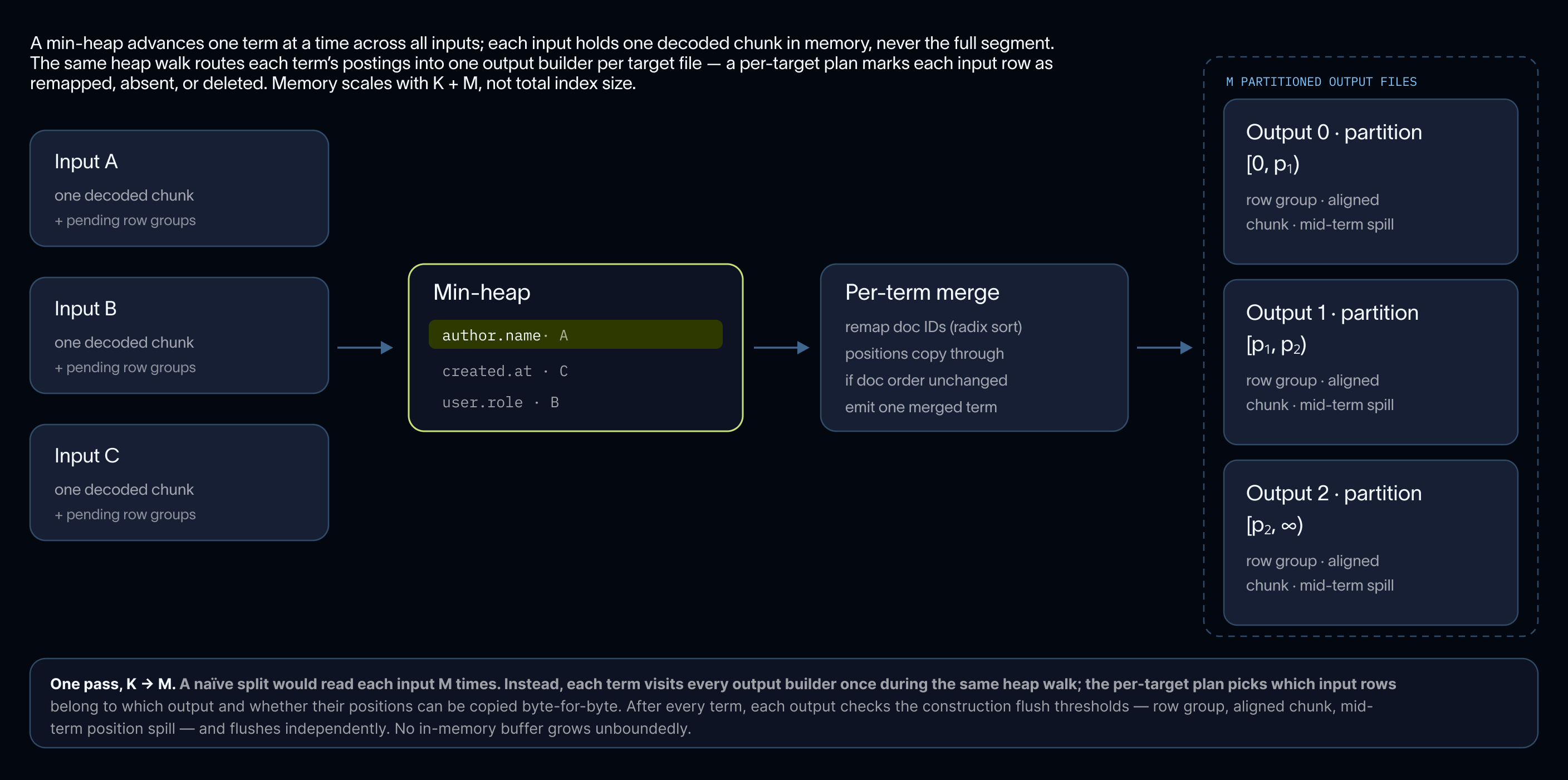
ミニヒープ(最小ヒープ)がすべての入力に対して用語ごとに 1 つずつ進みます。各入力は、常にメモリー上にデコードされたチャンクを 1 つだけ保持し、完全なセグメント全体を保持することはありません。マージされた用語はすでにソート済みで出力されます(FST の書き出しに必須)。また、構築時と同じ 3 つのフラッシュ閾値(ロウグループ、アラインされたチャンク、中間用語ポジションのスパイル)が、各用語処理後に出力ビルダーを制約します。メモリーは、関与するセグメントの数に関わらず、マージされる入力の数に比例してスケールし、インデックス全体のサイズには依存しません。
クエリ実行時
読み取りパスは、SmithDB の他のクエリが既に流れるのと同じ仕組み(DataFusion と Vortex の LayoutReader パイプライン)を再利用し、逆インデックスをプランナーが述語に押し込む別のレイアウトとして組み込みます。SQL 表面やクエリプランナーがインデックスの存在を学習する必要はありません:これらはすべて、当社の TableProvider および LayoutReader の実装によって内部で処理されます。
特定のクエリに対して、メタストアから候補セグメントを解決した後、プランナーは、その中で実際にクエリ対象の列に対してインデックスが構築されているセグメントを確認します。クエリ対象の列に対するインデックスを持たないセグメントは静かにカラムスキャンへルーティングされ、インデックスを持つセグメントはインデックスへルーティングされます。これらすべての処理は、オブジェクトストレージへの要求が行われる前に完了します。
One segment, many files
SmithDB では、各メタストアエントリは行データを保持する 1 つのコアファイルと、インデックス化された各列に対応する兄弟ファイルを指します。クエリ実行時の課題は、このファイル群を DataFusion(上位層)および IO スケジューラ(下位層)の両方に対して単一のアドレス可能エンティティとして振る舞わせつつ、各述語が実際に開く必要があるファイルを選択できるようにすることです(すべての述語がインデックスファイルのダウンロードと開封を必要とするわけではありません)。
計画時には、各述語はセグメントごとに 1 回だけ検査され、3 つの結果のいずれかにルーティングされます。すなわち、インデックスを通じて読み込む(このセグメントで列がインデックス化されている)、コアファイルでの列スキャンにフォールバックする(インデックスが存在しない)、または「一致なし」へショートサーキットする(列が投影されていない)のいずれかです。これら 3 つの決定は、すべてのオブジェクトストレージ要求の前に行われます。そのため、クエリ対象列に対してインデックスを持たないセグメントではインデックスファイルが開かれず、ある述語に対してインデックスを持つセグメントではその述語に対応する列が開かれません。
実行時には、コアファイルと各インデックスファイルが単一の仮想レイアウトを構成します。DataFusion は 1 つの論理ファイルセグメントとして認識し、投影プッシュダウン(projection pushdown)、述語プッシュダウン(predicate pushdown)、およびセグメントの行インデックス空間が、コア列とインデックス列全体で均一に機能します。一方、IO スケジューラは各基盤ファイルからの実際のバイト範囲を認識するため、同じファイル内での読み込みは隣接する場合は自然に統合され、そうでない場合は正しくパーティション化されたまま維持されます。
100 列のうち 3 列にアクセスするクエリは、正確に 3 つのインデックスファイルを開きます。インデックスを使用しない述語は、インデックスファイルを全く開きません。ある列に対してインデックスが存在しないセグメントは、その列のみをスキャンする形で透明にフォールバックし、クエリの残りの部分に対するインデシング機能は無効化されません。
SmithDB の SQL 表面(json_key, json_key_search, search)は、プランナーによって Vortex 式へ書き換えられ、時間範囲、投影、およびコアファイルへの結合はすべて変更されていない DataFusion プランとして実行されます。以前のブログ記事で記述した v1→v2 レイアウト移行 には、Vortex レイヤーより上での変更はゼロでした:同じ式インターフェースですが、その下のバイト列が異なります。
レイアウトから GET へ
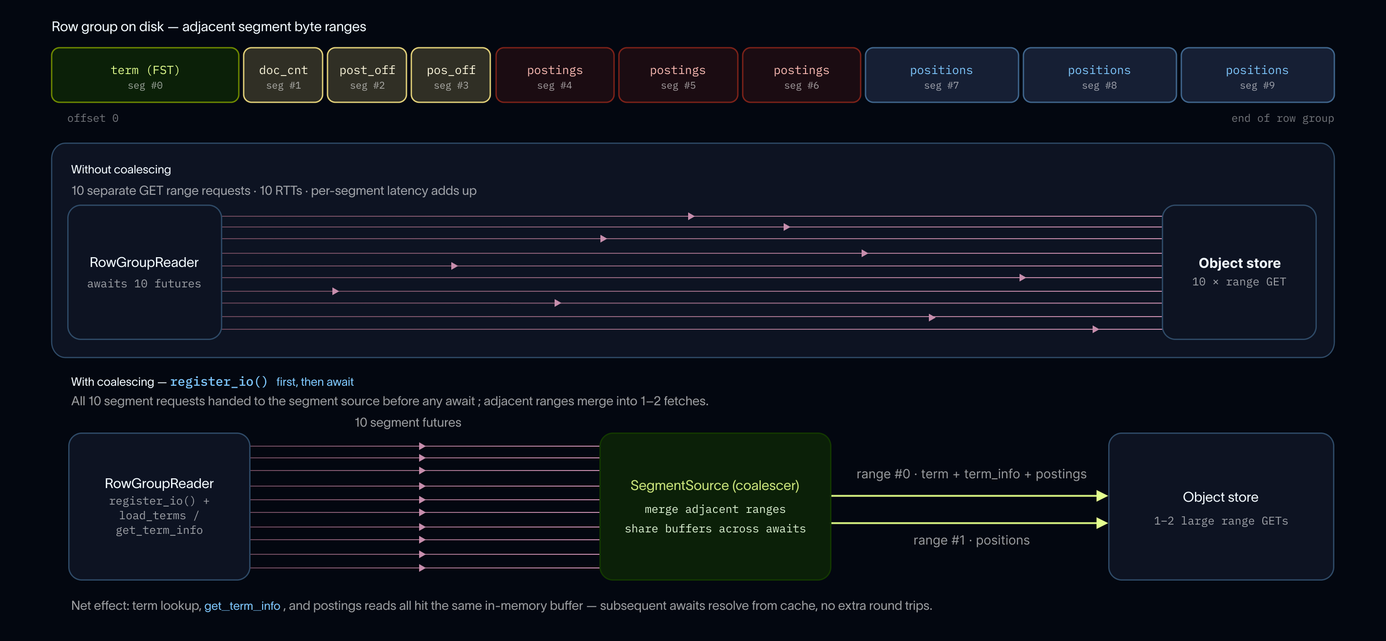
以前のブログ記事では、逆インデックスデータをどのように行グループに整理しているかを概説しました。各行グループの読み込みには 2 つのフェーズがあります:範囲登録とデコードです。リーダーは用語を FST(Finite State Transducer)に対して解決し、その term_info エントリを読み込んで投稿(句クエリの場合は位置情報も)オフセットおよび長さを取得し、オブジェクトストアへの要求を発行する前に必要なすべての範囲を Vortex セグメントスケジューラに登録します。スケジューラは隣接する範囲をマージし、最大 1 MB のギャップで隔てられた非隣接範囲を結合し、統合されたウィンドウを 16 MB に制限します。
オブジェクトストレージでは、各 GET リクエストには固定の per-request latency とコストが発生し、小規模な読み取りにおいてはこれが支配的となるため、リクエスト数が重要になります。Coalescing はわずかな転送の無駄(1 MB 未満のギャップ部分)を犠牲にしてラウンドトリップ回数を減らすものであり、用語の範囲が物理的に近接しているレイアウトであるためここでは効果的です:行グループは 32 MB の postings バジェットによって制限され、postings と positions は共有ドキュメント境界にアライメントされた約 2 MB チャンクでフラッシュされます。選択的な用語に対するフレーズ検索は、term_info、postings、positions をすべてカバーする単一の GET に解決されます。一方、非フレーズ検索は term_info と postings をカバーする単一の GET に解決されます。単一の GET は用語の頻度に関わらず行グループバジェットによって上限が設定されています。
一度行グループの範囲がフェッチされると、デコードは返されたバッファ内だけで完結し、オブジェクトストアへの追加のリクエストは発生しません。シークもローカルで行われます:ブロックビットパック形式のデルタは、各ブロックごとのビット幅をインラインで記録しているため、ブロックをスキップしてもカーソルが一定のオフセット分だけ進み、デコードする必要もなく GET を発行することもありません。したがって、クエリが行うオブジェクトストアへの要求は、行グループごとの読み取り自体のみです。そのため、クエリのレイテンシはプルーニング後に残存する行グループの数によって上限が決定され、各 GET は行グループのバイトバジェットによって制限されます。100 ミリ秒のラウンドトリップは、まさにその回数だけレイテンシ予算に組み込まれます。
3 つのクエリ形状と 3 つのルックアップパス
ルーティングが述語をインデックスレイアウトに渡した後、3 つの クエリ形状 のそれぞれが、v2 カラム(term, term_info, postings, positions)に直接マッピングされます。
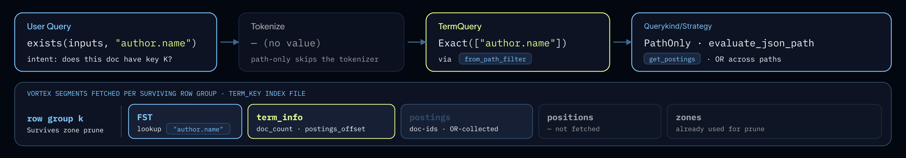
パスのみ (json_key) は term_key FST を走査して postings を返します。これはフレーズクエリではないため、positions は決して読み込まれません。復号化された postings は、親レイアウトリーダーがフィルタリングに使用する行インデスマスクとなります。これは 3 つの形状の中で最も安価なものであり、ゾーンレベルのプルーニングが最も効果を発揮するケースです:プレフィックスパターンを持つパスクエリ (json_key(inputs, "author.%")) は、通常、FST の処理が行われる前にほとんどの行グループをスキップします(私たちの FST はパーティション化されています)。
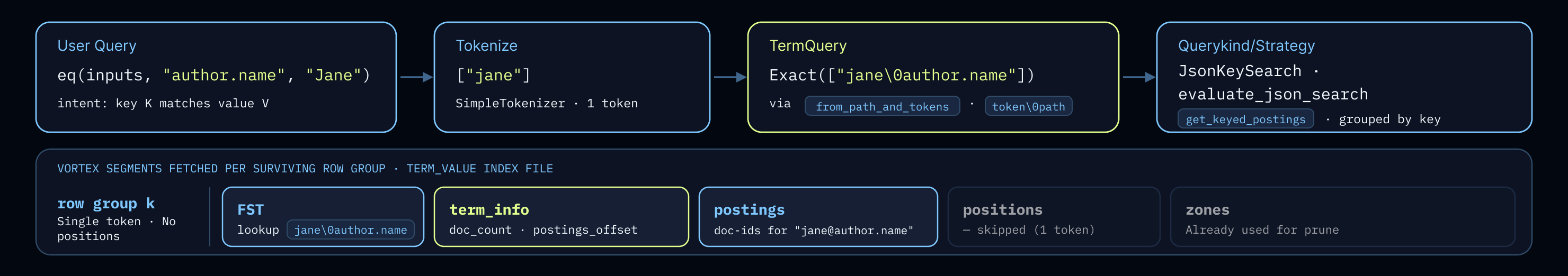
キー付き検索 (json_key_search) は、v2 レイアウトで導入された token\0path キーイングを使用して、term_value に対して 1 つ以上の FST ルックアップを実行します。単一トークンのルックアップは、単一の FST 完全一致と単一の postings フェッチです。複数トークンのフレーズバリアントでは、まず postings の共通部分を求めた後、隣接性をチェックするために PhraseQuery にフォールスルーします。
フルテキスト検索では、同じ term_value FST が 2 つのモードで再利用されます。プレーンテキスト列の場合は完全一致による照合が行われます。一方、JSON 値に対する自由テキストについては、token\0 プレフィックススキャンがトークンが存在するすべてのパスを走査し、それぞれの投稿リスト(postings)を結合します。これにより、キー付き検索とキーなし検索の両方を単一の FST で処理でき、辞書はもう一つ必要なく、追加の入出力も不要です。
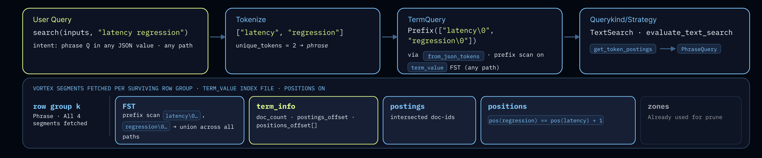
3 つの形状のいずれにおいても、マルチトークンフレーズは PhraseQuery を経由して処理されます。これは 2 つの段階で動作します:まず投稿リストを交差させて候補ドキュメントを絞り込み、次にその候補のみに対して位置情報を復号化して隣接性を検証します。位置情報の復号化は投稿リストの交差演算に依存しているため、一致するドキュメント数が少ないフレーズ照合では、ほぼ位置情報に関する入出力が発生しません。この非対称性が、別個の位置情報列を設計した目的そのものです。
最近取り込まれたデータの処理
観測性(observability)クエリは強く直近のデータに偏っており、顧客はデバッグのために自分が直近で取り込んだトレースが数秒以内に検索可能であることを期待します。前節で説明した「取り込み中にインラインで構築されるインデックス」という構成モデルがこれを可能にしますが、これには読み取りパスが 2 つのストレージ階層を跨ぐ必要があります:
- L0: 取り込みノード上のローカル SSD。取り込みサービスがバッチのランを処理して取り込む際、そのバッチに対する列ごとの逆インデックスはオブジェクトストレージに永続的に書き込まれるのではなく、ローカル SSD に書き込まれます。そのため、「トレースコミット」から「L0 インデックスが利用可能になるまで」のレイテンシは非常に高速です。
- L1: オブジェクトストレージ。取り込みサービスによるベストエフォート型のコンパクションにより、L0 セグメントとそのインデックスがオブジェクトストレージへプロモートされます。取り込みサービスで処理しきれなかったものは、必要に応じてインデックスを再構築するものも含め、専用のコンパクションサービスによって引き継がれます。
クエリ実行時のルーティングにより、両階層の整合性が調整なしに保たれています。当社のクラスターマネージャーはすでにスティッキールーティング(sticky routing)を実装しており、特定のテナントおよびトレーシングプロジェクトに対するクエリは、そのスコープに対して最も最近書き込みを行ったノードへ送信されます。そのため、最新のクエリはライターノードに到達し、レイアウトリーダー(LayoutReader)がそのノード上のメモリエディット L0 インデックスと、より古いセグメントの L1 インデックスを合成します。これは他の場所と同じ LayoutReader ツリーですが、一部の子要素がオブジェクトストレージではなくローカル SSD を指している点が異なります。過去 1 時間全体にわたるクエリは、ライターノードでの L0 リードとオブジェクトストレージでの L1 リードを透明に混合しますが、SQL サーフェスも述語ルーティング(predicate routing)も変更されません。
「ライブテール」モードという別機能はなく、最終的に整合性が取られるまでのギャップも存在しません。L0 を別のシステムとして並列に構築するのではなく、同じインデックスの追加階層として扱うことで、サブ秒単位の鮮度を実現しています。
次のステップ
今後間もなく、フルテキスト検索および逆インデックス実装に対して多くの最適化を行い、文書化する予定です。さらに、ストレージレイアウトの最適化と分散クエリ実行を組み合わせることで巨大なデータセット上でサブ秒単位の統計情報をどのようにサポートしているかといった、SmithDB の内部構造に関するブログ記事も追加で執筆する予定です。
//
*私たちは、エージェントの観測性に伴うシステム課題を解決するために SmithDB を構築しています。このようなインフラストラクチャ開発に興味をお持ちであれば、*採用情報はこちら*です。*
関連コンテンツ
LangChain のシステム
SmithDB におけるフルテキスト検索:オブジェクトストレージ向け逆インデックスの設計


A. Gola,
A. Aurora,
S. Arani
2026 年 6 月 10 日
15 分

エージェントの実際の動作を確認する
LangSmith は、エージェントエンジニアリングプラットフォームであり、開発者がすべてのエージェントの意思決定をデバッグし、変更の評価を行い、ワンクリックでデプロイできるように支援します。
原文を表示
Full Text Search in SmithDB: Constructing and Querying our Inverted Index (Pt. 2)
Overview
In our earlier blog post on supporting full text search in SmithDB, we went over how we designed our object-storage backed inverted index implementation. In this blog post, we will cover how we construct, compact, and query this index in SmithDB.
Inverted index construction and merging
Index construction happens inline during ingestion. New runs become searchable within seconds, and because the freshest data is still resident on the node that wrote it, leading-edge queries read both the indexes and core data files directly from local storage instead of paying a round trip through object storage. On compaction, we merge indexes associated with different data files.
Payload parsing
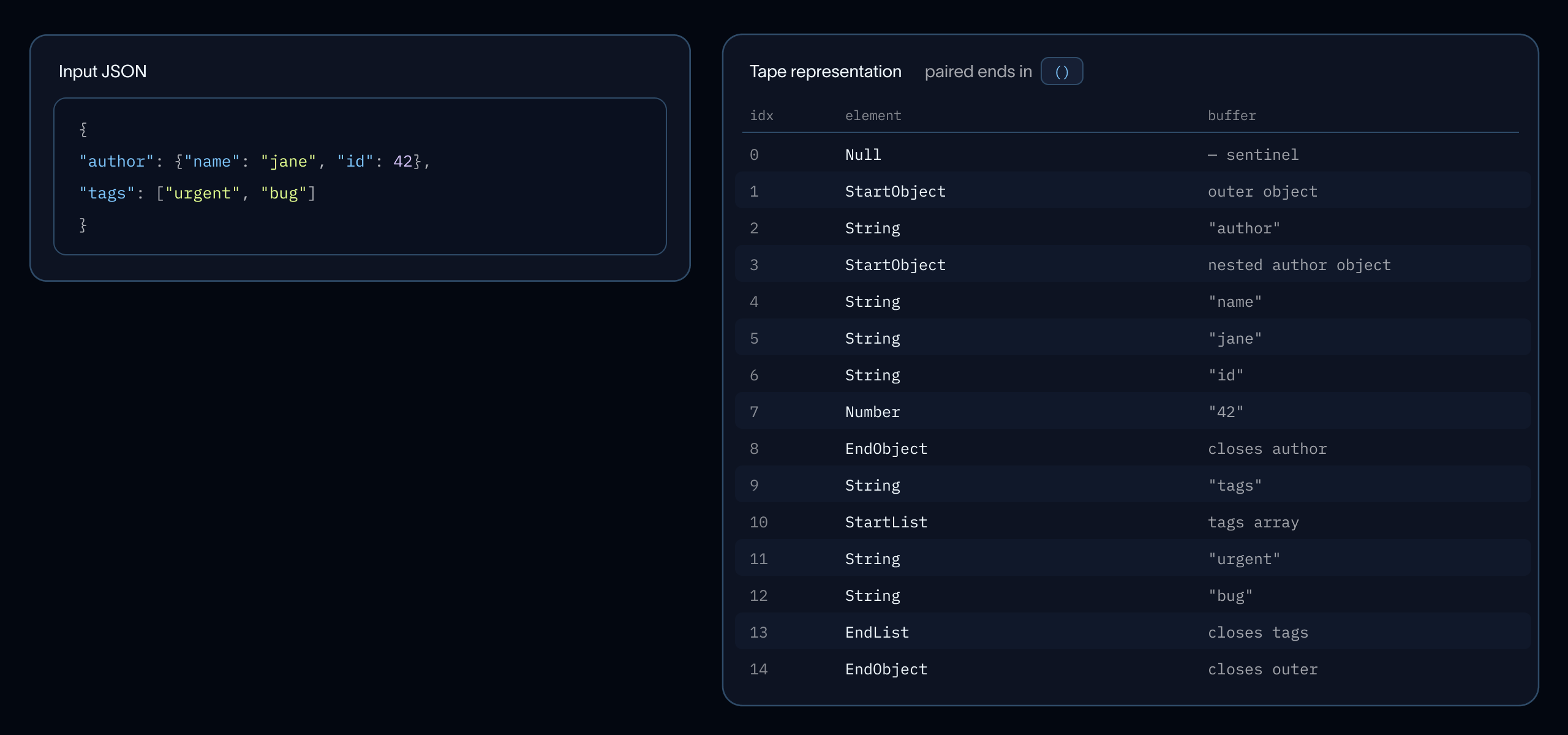
Recall that SmithDB indexes the large inputs and outputs fields (among a few others) present in run payloads. For deeply nested and large payloads, JSON parsing dominates construction time. We only need flattened key paths and leaf values, so we built a JSON tape adapted from Apache Arrow's arrow-json crate, which is itself inspired by simdjson's tape format.
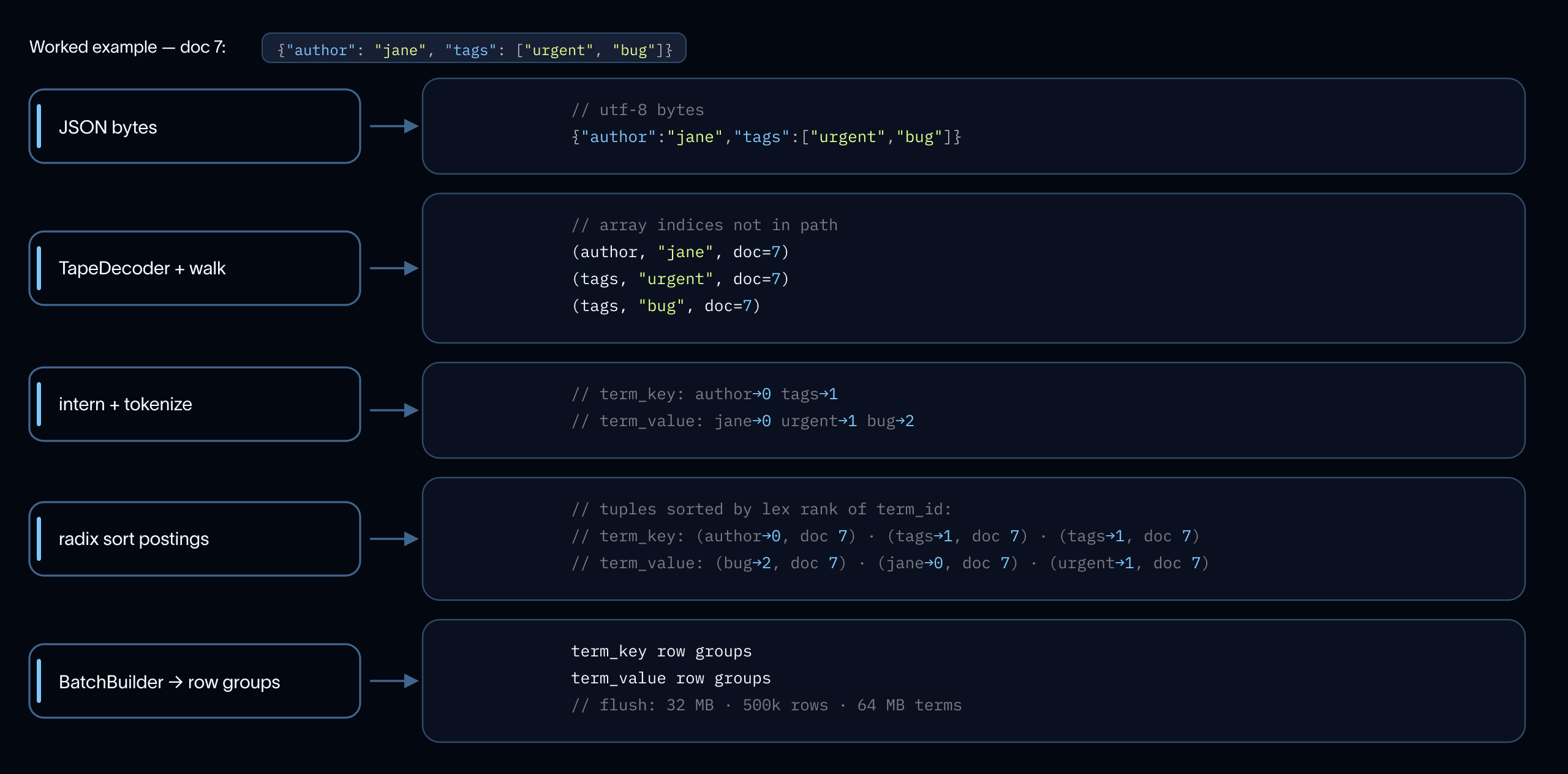
Our implementation consists of a flat sequential array of tokens with all string bytes in one contiguous buffer: no per-field allocation, no numeric conversion. A single-pass iterator then flattens each document into (path, leaf_value) pairs: nested objects become dotted paths, array elements collapse onto their parent key: {"agent": "deep agents", "tags": ["langchain", "engine"]} yields (agent, "deep agents"), (tags, "langchain"), (tags, "engine").
See below for another example.
Tokenization
Before a value becomes an index term, it is tokenized: split on non-alphanumeric boundaries, lowercased, dropped of stop words, and capped at 256 characters.
Sorting and interning
Recall that we use finite state transducers (FSTs) for our term layout in our inverted index implementation. The flat postings table must be sorted by term before it can feed the FST writer.
Across agent traces, the same JSON paths and token values repeat in virtually every document for a particular tenant and tracing project. When implemented naively, this sort is dominated by string comparisons. To get around this, we leverage string interning: a technique that maps each unique term to a compact integer ID upfront. As a result, comparison cost scales with distinct terms, not occurrences, cutting construction time by ~2.2× in our benchmark.
We use ahash for hashing (stdlib ~20% slower, Tantivy's MurmurHash2 ~30% slower), store all bytes in one contiguous buffer, and use Hashbrown's raw API to hash each string exactly once per intern call. Each occurrence is then recorded as a (doc_id, term_rank, position) triple in a flat table. We leverage radix sort to group postings by term in O(n) before the sorted run feeds the FST writer.
Flush thresholds
Accumulating an entire batch before writing would let a single high-frequency term (5, agent, or a common JSON key) grow unboundedly. During index write, we have optimized flush boundaries on three thresholds:
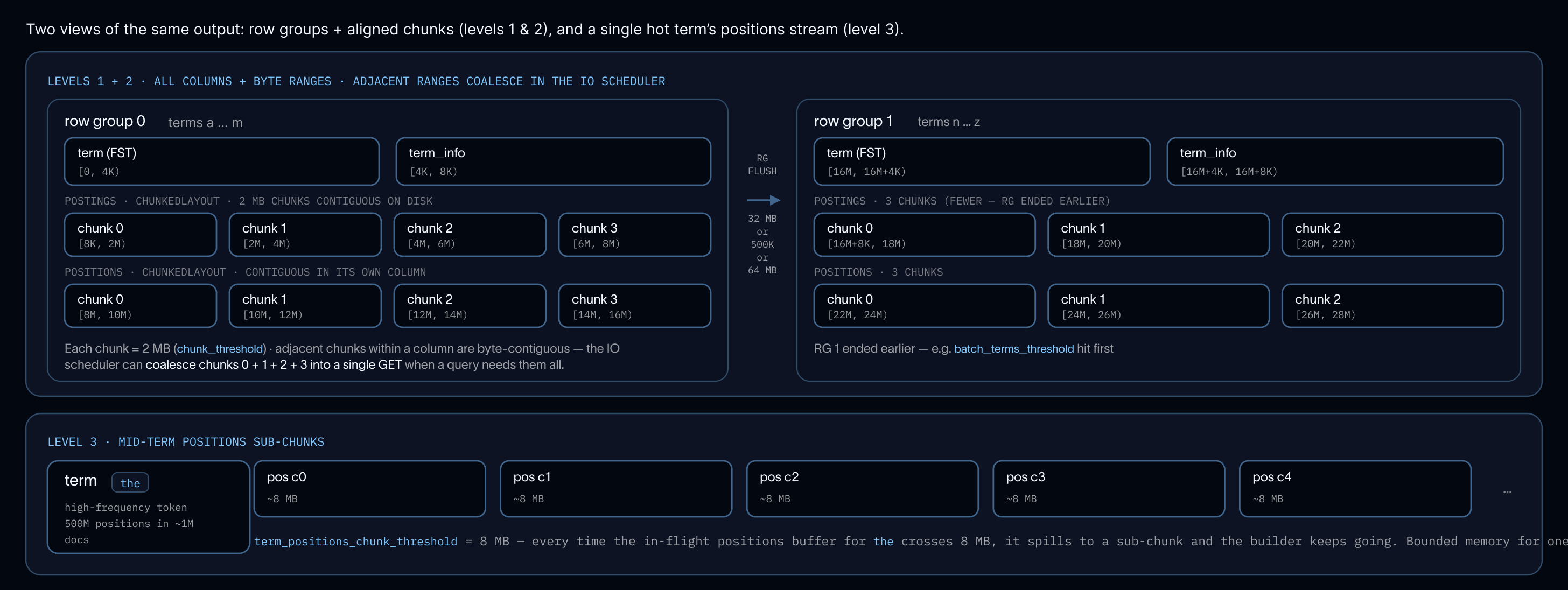
- a row group: 32 MB postings / 500 K terms / 64 MB raw term bytes, sized to keep the in-memory FST writer within addressable memory
- an aligned chunk: ~2 MB, postings and positions flush at matching document boundaries so a query reading both gets contiguous byte ranges in a single GET
- a mid-term position spill: 8 MB, an escape hatch for Zipfian tail terms like 5 that would otherwise accumulate hundreds of millions of positions before the term finishes
Chunks within each column are byte-contiguous on disk, so every threshold maps directly to a worst-case GET size and a worst-case memory footprint.
Index merge
Our compaction service merges smaller files written by ingestion into larger files more optimal for querying. Along with compacting core files, the service processes each core file’s per-file indexes with a streaming merge.
A min-heap advances one term at a time across all inputs; each input holds only one decoded chunk in memory at a time, never the full segment. The merged terms emerge already sorted (required by FST writing) and the same three flush thresholds from construction (row group, aligned chunk, mid-term position spill) bound the output builder after every term. Memory scales with the number of inputs being merged, not the total index size, regardless of how many segments are involved.
Query time
The read path reuses the same machinery the rest of SmithDB queries already flow through (DataFusion and Vortex's LayoutReader pipeline) and slots the inverted index in as another layout that the planner pushes predicates into. Nothing about the SQL surface or the query planner had to learn that an index exists: it’s all handled internally by our TableProvider and LayoutReader implementations.
For a given query, after resolving the candidate segments from our metastore, the planner checks which of those segments actually have an index built for the column being queried. Segments missing an index for the queried column are quietly routed to a column scan instead; segments with an index are routed to the index. All of this happens before any object-storage request.
One segment, many files
In SmithDB, each metastore entry points to one core file holding the row data, plus a sibling file per indexed column. The challenge at query time is making this collection of files behave like a single addressable entity (both to DataFusion above and to the IO scheduler below) while still letting each predicate pick which files it actually needs to open (not all predicates require downloading and opening index files).
At plan time, each predicate is inspected once per segment and routed to one of three outcomes: read it through the index (the column is indexed in this segment), fall back to a column scan on the core file (no index available), or short-circuit to "no matches" (the column isn't projected at all). All three decisions are made before any object-storage request, so a segment with no index for the queried column never opens an index file, and a segment with one never opens the column for that predicate.
At runtime, the core file and each index file compose into a single virtual layout. DataFusion sees one logical file segment: projection pushdown, predicate pushdown, and the segment's row-index space all work uniformly across core and index columns. The IO scheduler, on the other hand, sees the actual byte ranges from each underlying file, so reads inside the same file coalesce naturally where they're adjacent and stay correctly partitioned where they aren't.
A query that touches three columns out of a hundred opens exactly three index files. A predicate that doesn't use the index never opens an index file at all. A segment that's missing an index for one column transparently falls back to a scan for *just that column*, without disabling indexing for the rest of the query.
The SmithDB SQL surface (json_key, json_key_search, search) is rewritten by the planner into a Vortex expression; time bounds, projections, and joins to the core file all run through unchanged DataFusion plans. The v1→v2 layout migration we described in our earlier blog post required zero changes above the Vortex layer: same expression interface, different bytes underneath.
From layout to GETs
Our earlier blog post outlined how we organize our inverted index data into row-groups. Each row-group read has two phases: range registration, then decode. The reader resolves the term against the FST, reads its term_info entry to obtain postings (for phrase queries, positions as well) offsets and lengths, and registers all required ranges with the Vortex segment scheduler before issuing any object-store request. The scheduler merges adjacent ranges, combines non-adjacent ranges separated by gaps of up to 1 MB, and caps the coalesced window at 16 MB.
On object storage, each GET carries fixed per-request latency and cost that dominate for small reads, so the number of requests matters. Coalescing trades a little wasted transfer (the sub-1 MB gaps) for fewer round trips, and it's effective here because the layout keeps a term's ranges physically close: row groups are bounded by a 32 MB postings budget, and postings and positions flush in ~2 MB chunks aligned on shared document boundaries. A phrase lookup against a selective term resolves to one GET covering term_info, postings, and positions; a non-phrase lookup resolves to one GET covering term_info and postings. A single GET is bounded above by the row-group budget regardless of term frequency.
Once a row group's ranges are fetched, decode happens entirely within the returned buffer, with no further object-store requests. Even seeking is local: block-bitpacked deltas record their per-block bit width inline, so skipping a block advances the cursor by a constant offset without decoding it and without issuing a GET. So the only object-store requests a query makes are the per-row-group reads themselves. Query latency is therefore bounded by the number of row groups surviving pruning, with each GET bounded by the row-group byte budget. The 100 ms round trip enters the latency budget exactly that many times.
Three query shapes, three lookup paths
Once routing has handed the predicate to the index layout, each of the three query shapes maps directly onto the v2 columns (term, term_info, postings, positions).
Path-only (json_key) walks the term_key FST and returns postings. Positions are never read since this isn’t a phrase query. The decoded postings become a row-index mask the parent layout reader uses for filtering. This is the cheapest of the three shapes and the one zone-level pruning helps most: a prefix-pattern path query (json_key(inputs, "author.%")) typically skips most row groups before any FST work happens (our FSTs are partitioned).
Keyed-search (json_key_search) does one or more FST lookups against term_value, using the token\\0path keying introduced in the v2 layout. A single-token lookup is a single FST exact-match plus a single postings fetch. Multi-token phrase variants intersect postings first, then fall through to PhraseQuery for adjacency.
Full-text (search) reuses the same term_value FST in two modes. For plain-text columns it's an exact lookup. For free-text over JSON values, the token\\0 prefix scan walks every path the token appears under and unions their postings: one FST serving both keyed and unkeyed search, no second dictionary, no extra IO.
Multi-token phrases on any of the three shapes run through PhraseQuery, which works in two stages: first intersect postings to narrow the candidate documents, then decode positions only for those candidates and verify adjacency. Because position decode is gated behind the postings intersection, a phrase query that matches few documents pays almost no positions IO. That asymmetry is exactly what the separate positions column was designed to enable.
Handling recently ingested data
Observability queries skew hard toward recent data, and customers expect a trace they just ingested to be searchable within seconds for debugging. The "indexes built inline during ingestion" construction model from the previous section is what makes that possible, but it requires the read path to span two storage tiers:
- L0: local SSD on the ingestion node. When ingestion accepts a batch of runs to ingest, the per-column inverted index for that batch is written to local SSD, not durably to object storage. Latency from "trace committed" to "L0 index visible" is therefore very fast.
- L1: object storage. A best-effort compaction in the ingestion service promotes L0 segments and their indexes to object storage; anything ingestion doesn't get to is picked up by the dedicated compaction service, including reconstructing indexes where necessary.
Routing at query time keeps the two tiers coherent without coordination. Our cluster manager already does sticky routing: queries for a given tenant and tracing project go to the node that most recently wrote for that scope. So leading-edge queries land on the writer node, where the layout reader composes that node's in-memory L0 indexes alongside the L1 indexes for older segments. It's the same LayoutReader tree as everywhere else, just with some children pointing at local SSD instead of object storage. A query spanning the last hour transparently mixes L0 reads on the writer node with L1 reads on object storage, and neither the SQL surface nor the predicate routing changes.
There's no separate "live tail" mode and no eventually-consistent gap. Sub-second freshness results from treating L0 as one more tier of the same index, rather than building a parallel system to serve it.
What’s next
We’ll be making and documenting quite a few optimizations to our full text search and inverted index implementation in the near future. Additionally, we’ll be writing more blog posts on SmithDB internals including how we support sub-second stats on massive datasets through a combination of storage layout optimizations and distributed query execution.
//
*We’re building SmithDB to solve the systems problems that come with agent observability. If that kind of infrastructure work sounds interesting, *we’re hiring*.*
Related content
Systems at LangChain
Full Text Search in SmithDB: Designing an Inverted Index for Object Storage
A. Gola,
A. Aurora,
S. Arani
June 10, 2026
15
min
See what your agent is really doing
LangSmith, our agent engineering platform, helps developers debug every agent decision, eval changes, and deploy in one click.
関連記事
AI エージェントに記憶機能を実装する方法
LangChain が、AI エージェントに長期・短期の記憶機能を組み込むための具体的な手法とアーキテクチャを解説している。
AWS で現代的なデータメッシュ戦略を用いたエージェント型 AI アプリケーションの構築
AWS は、顧客サービスエージェントが自律的にデータベースを照会し回答を合成する際、組織内の複数のデータソースにまたがるガバナンスアクセスが必要であると指摘。現代のデータメッシュでは、データ相互作用チェーンの各層で厳密なアクセス制御を適用することが重要であるとしている。
2026 年に AI エンジニアになるためのロードマップ
KDnuggets が、2026 年までに AI エンジニアとして活躍するための学習ロードマップを提示している。
今日のまとめ
AI日報で今日の重要ニュースをまとめ読み