CMU、多期間予測のボラティリティ低減手法「Forking-Sequences」を論文とコード公開
本文の状態
日本語全文を表示中
詳細モードで約14分の本文を読めます。
同じ出来事の情報源
この情報源を基点に整理
ML@CMU
CMU の研究チームは、Forking-Sequences 手法に基づく時系列予測モデルにおいて、推論時のアンサンブルにより volatilty を大幅に低減しつつ精度を維持する新手法を発表した。
Continue in AI NEW LAB
このニュースを、実務の判断につなげる
AI NEW LABで、試したことや先に確認したい条件を共有できます。まずはログインなしで読めます。
AI NEW LABで論点を見るAI深層分析を開く2026年8月11日 07:32
AI深層分析
キーポイント
計算コスト増なしの予測安定化
Forking-Sequences は単一順次パスで全ての予測日に対する重複 forecasts を生成するため、推論時にアンサンブルを適用しても追加のエンコーダー計算が必要にならない。
新しい変動性評価指標の導入
Ground truth 不要でリアルタイムの修正規模を測る sFPC と、精度向上に寄与する修正は称賛し誤った方向への修正や過剰反応のみを罰する Excess Volatility (EV) の2つの新指標が提案された。
既存モデルへのゼロショット適用
Chronos-2 や TimesFM などの事前学習済み時系列ファウンデーションモデルに対して、追加学習なしでアンサンブル手法を適用することで変動性を約10%削減し、精度低下は0.1%未満に抑えた。
Forking-Sequencesによる自然なアンサンブル
この手法は単一の順方向パスで各FCDの予測を生成するため、同じ対象日に対する複数の重複する予測が得られる。これにより、推論時にエンコーダー計算を再利用して追加コストなしで予測アンサンブルが可能となる。
予測変動性の低減と有用な改訂の識別
目標は改訂を完全に排除することではなく、有益な情報に基づく改訂と根拠のない erratic な改訂を区別することにある。アンサンブル手法によりFCD間での予測変動性が減少し、より安定した分布が得られる。
重要な引用
Ensembling, nearly for free.
Exponential-smoothing forecast ensembling (α = 0.9) reduces sEV by 10–13% across all encoder types, with less than 0.1% accuracy degradation.
The goal isn't to eliminate revisions, it's to distinguish benign, informative revisions from excessive, erratic ones.
By reusing encoder computations, forking-sequences enables computationally efficient forecast ensembling with negligible additional cost.
編集コメントを表示
編集コメント
この研究は、時系列予測の実用化における最大の課題の一つである予測の不安定さを、アーキテクチャの特性を最大限に活用することで解決する道筋を示している。既存のファウンデーションモデルに対する適用可能性が高い点は、現場での即戦力としての期待値を高める要素と言える。
Source Article
元記事を日本語で読む
本文に関係しない購読案内、埋め込み通知、サイト内プロモーションは除いています。
出典:Potosnak, W., Wolff, M., Cao, M., Ma, R., Konstantinova, T., Efimov, D., Mahoney, M.W., Oreshkin, B., & Olivares, K.G.「Forking-Sequences: Statistically and Computationally Efficient Multi-Horizon Forecasting with Reduced Volatility」Transactions on Machine Learning Research, 2026.

(免責事項:本論文で使用されたコード実装ではありません。Amazon とは関係ありません。Forking-Sequences および予測アンサンブルの参考資料として提供されています)
TL;DR
アンサンブル処理をほぼ無償で実現可能。Forking-Sequences は、単一の順方向パスで FCD(Future Context Dates)上のすべての対象日に対して重複する予測を生成するため、推論時にこれらをアンサンブルしても、ウィンドウサンプリングと比較してエンコーダーの計算コストは追加されません。
2 つの新しい予測変動性指標。スケーリングされた予測パーセント変化(sFPC)は、実時間での生修正サイズを測定します(正解データは不要)。一方、Excess Volatility(EV)はさらに一歩進み、精度向上につながる修正には報酬を与え、真値から遠ざかる修正や過剰な修正に対してのみペナルティを科します。
精度を犠牲にせず変動性を低減。指数平滑化による予測アンサンブル(α = 0.9)は、すべてのエンコーダータイプで sEV を 10〜13% 削減し、精度の低下は 0.1% 未満です。
ウィンドウサンプリングで事前学習されたモデルに対して、ゼロショットで動作します。時系列ファウンデーションモデル(TSFMs)である Chronos-2、Toto 2.0、TimesFM、PatchTST、N-BEATS に予測アンサンブルを適用すると、精度への影響はほぼゼロ(0.1%未満)でありながら、変動性を約 10% 削減できます。
パート I では、フォークシーケンスというニューラルネットワークのアーキテクチャを紹介しました。これは、すべての予測作成日(FCDs)にわたって時系列を同時に符号化・復号化するもので、単一の順方向パスで完結します。これがなぜウィンドウサンプリングよりも統計的かつ計算効率的な学習パラダイムなのかを示しました。パート II では、同じく重要な問題である予測の変動性(volatility)に焦点を当てます。
なぜ予測変動性が重要なのか
予測モデルの評価では精度が最も注目される指標ですが、実運用においてそれが唯一の基準ではありません。多期間予測システムは時間経過とともに動作するため、将来のある特定の日付に対して複数の重複する予測を生成します。これは、より多くのデータが利用可能になるたびに新しい FCD から一つずつ出力されるものです。この一連の更新を「予測修正」と呼びます。これらの修正がいかに一貫しているか(あるいは不規則であるか)こそが、私たちが定義する予測変動性です。
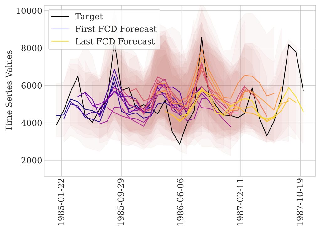 image(a) 予測推論アンサンブルなし
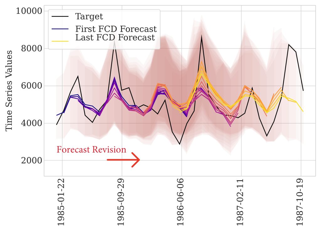 image(b) 予測推論アンサンブルあり
図 1: (a) フォーカスト・アンサンブルを適用しない場合と、(b) 適用した場合の予測比較。予測アンサンブルは異なる FCD(Future Context Duration)間で予測の変動性を低減し、より安定した一貫性のある予測分布を実現します。赤い矢印は予測修正の方向を示しています。各線は、異なる FCD にわたる P50(中央値)予測を表しています。エンコーダー計算を再利用することで、Forking-Sequences は追加コストを実質ゼロに抑えつつ、計算効率の高い予測アンサンブルを可能にします。
電力系統の運用者が負荷予測を用いて供給計画を立てている状況を想像してください。例えば、猛暑が迫る前に予測値が 45 GW から 65 GW に修正された場合、これは有用な修正です。運用者は予備発電所の稼働を指示できます。しかし、新しい情報を根拠とせずに FCD を跨いで予測値が不安定に跳ね回るようであれば、信頼性が損なわれ、計画立案は複雑化します。目指すべきは修正そのものを排除することではなく、有益で情報量の多い修正と、過度で不規則な修正を見分けることです。
これにより、本論文で直接取り組む 2 つの問いが浮かび上がります:
- 有用な修正と有害な修正を明確に区別し、予測の変動性を測定する方法は何か?
- 精度を損なうことなく変動性を低減できるアーキテクチャ設計は存在するか?
Forking-Sequences を自然な予測アンサンブルメカニズムとして
Forking-sequences は、単一の順方向パスで FCD(Forecast Cut Date)ごとに予測を生成するため、同一の目標日に対して複数の重複した予測が自然に得られます。前述の通り、予測の改訂関係は以下のようになります:FCD t+1 で行われたある目標日に対する予測は、FCD t で同じ日付に対して行われた予測の改訂版です。Forking-sequences パラダイムにおける予測の改訂例を Fig. 2 に示します。
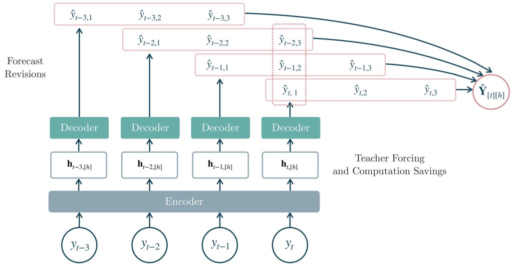 imageFig. 2: Forking-sequences
この重複するグリッド構造により、Forking-sequences モデルは、複数の独立したモデル順方向パスを必要とする window-sampling に比べて、推論時にエンコーダー計算量を節約しながら、無料で(あるいはほぼ無料で)アンサンブル化できます。Forking-sequences を通じて得られた予測出力に対しては、Fig. 3a で対角バンドとして描かれている同一の目標日に対する異なる FCD レベルの予測を単純に平均する(または他の方法で結合する)だけでよいのです。
\[
\begin{equation}
\widetilde{\mathbf{Y}}_{t,h} = \frac{1}{H}\sum_{k=0}^{H} \widehat{\mathbf{Y}}_{t-k, h+k} \qquad \text{for } t\geq H.
\label{eq:forking_sequences_ensemble}
\end{equation}
\]
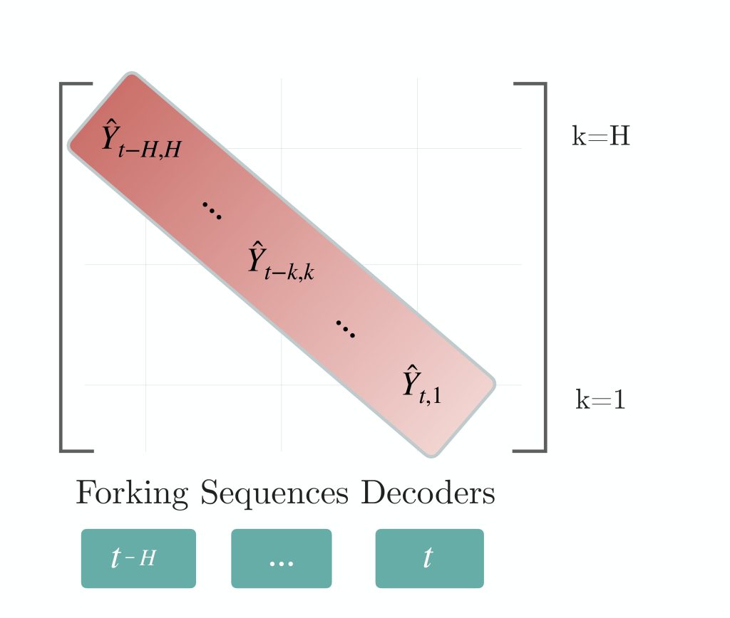 image(a) Forking-sequences 予測アンサンブル
 image(b) 予測のボラティリティ低減
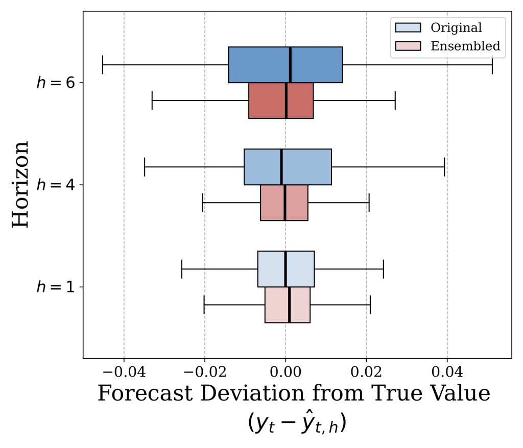
図 3: 推論時にフォークシーケンスを適応させ、過去の FCD から生成された予測に対して移動平均などの関数を計算することで、同一の未来日付に対する複数の予測をアンサンブルします。b) フォークシーケンスによるアンサンブルは予測のボラティリティを低減し、大数の弱法則に類似した線形収束率で推定値の分散を削減します。
定理 1 の結果と同様の分散低減効果を期待したくなるのは当然ですが、予測が対応する観測データから離れるほど予測誤差の分散は自然に増大するという事実を認識しておく必要があります。その結果、アンサンブルによるボラティリティ低減には本質的な限界が存在します。古い予測改訂は不確実性が著しく大きい一方、新しい改訂の方が精度が高く変動も小さいからです。そのため、すべての改訂を等しく扱うのではなく、新しい予測に重きを置くアンサンブル手法が望ましいと言えます。
新しい予測ボラティリティ指標
連続する予測作成日における予測分位値の相対変化を測定し、時系列のボラティリティや予測修正率を定量的に把握するために、スケーリングされた予測パーセント変化(sFPC)を導入しました。sMAPE 指標に触発された sFPC は、現在の予測と過去の予測の両方に基づく対称的な分母を使用することで、数値的不安定性の問題を軽減しています [1]。この設計により、小さな予測値を扱う際の堅牢性が確保され、従来のパーセントベースの指標でよく見られるゼロ除算の問題も回避されます。
\[
\mathrm{sFPC}^{(q)}\left(\hat{\mathbf{y}}^{(q)}_{[b][t][h]}\right)
= \frac{200}{B \times T \times H} \sum_{b,t,h} \frac{|\hat{y}^{(q)}_{b,t+1,h}-\hat{y}^{(q)}_{b,t,h+1}|}{|\hat{y}^{(q)}_{b,t+1,h}| + |\hat{y}^{(q)}_{b,t,h+1}|} .
\]
連続する予測間の sFPC を計算すると、精度が明らかに向上する修正であっても、すべての修正を同様に望ましくないものとして扱ってしまいます。これを解決するため、確率的予測に対する指標であるスケーリングされた過剰ボラティリティ(sEV)も導入しました。この指標は、予測が真値から遠ざかる場合や、真値をオーバーシュートする場合の修正のみをペナルティとし、精度向上につながる修正とは区別して評価します。
sEV は以下のように定義されます。
\[
\mathrm{sEV}\left(\mathbf{y}_{[b][t][h]}, \hat{\mathbf{y}}_{[b][t][h]}\right) = \frac{\sum_{b,t,h} \mathrm{EV}(y_{b,t,h}, \mathbf{\hat{y}}_{b,t,h+1}, \mathbf{\hat{y}}_{b,t+1,h})}{\sum_{b,t,h} |y_{b,t,h}|}, \quad \text{where}
\]
EV(y, \mathbf{\hat{y}}_1, \mathbf{\hat{y}}_2) = \mathrm{QL}(\mathbf{\hat{y}}_2,\mathbf{\hat{y}}_1) - (\mathrm{QL}(y,\mathbf{\hat{y}}_1)-\mathrm{QL}(y,\mathbf{\hat{y}}_2)) \quad \text{かつ} \\
\mathrm{QL}_q(y, \hat{y}^{(q)}) = q(y-\hat{y}^{(q)})_+ + (1-q)(\hat{y}^{(q)}-y)_+ .
EV には論文で厳密に証明された、3 つの有用な性質があります。
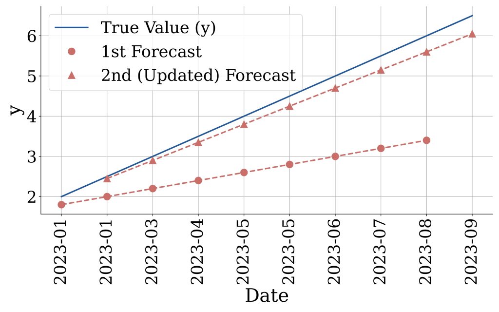
改善された修正に対するペナルティゼロ(図 4a):修正によって予測値が真値に対して比例的に近づき、真値と事前予測値を結ぶ直線上に乗った場合、EV は 0 になります。
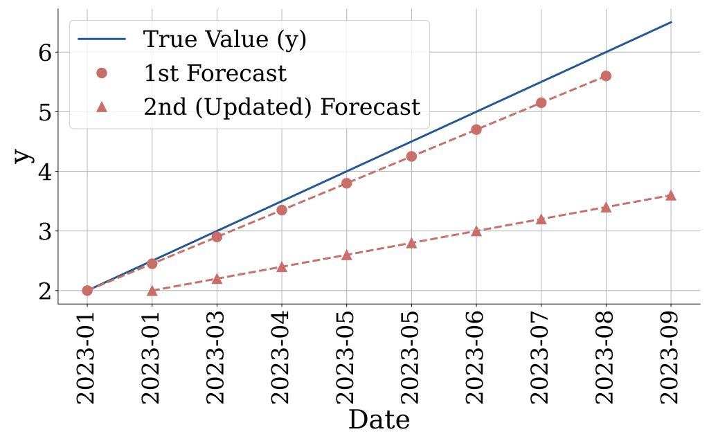
悪化した修正に対する最大ペナルティ(図 4b):修正によって予測値が真値から遠ざかり、かつ古い予測値が真値と新しい予測値の間に位置する場合、EV は完全な精度低下、すなわち新旧の予測値における分位点損失の差に等しくなります。
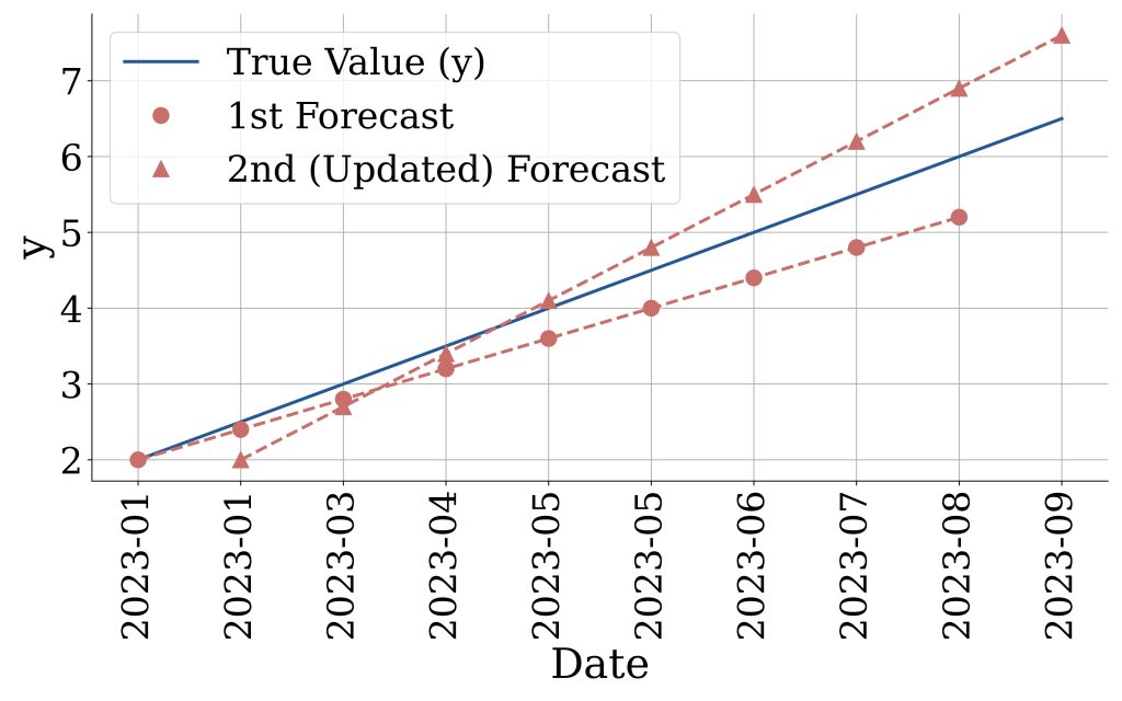
行き過ぎに対するペナルティ(図 4c):修正が正しい方向へ向かっているものの、真値を越えてしまい(真値が古い予測値と新しい予測値の間に入る)、その場合 EV は新しい予測値の真値に対する分位点損失のみを罰します。
 image(a) 改善された修正
 image(b) 悪化した修正
 image(c)Overshooting revision
図 4:Excess Volatility (EV) メトリクスのペナルティ挙動の例。EV は、精度を向上させる修正と精度を低下させる修正を区別します。精度が改善される場合はペナルティを与えず、逆に精度が低下したり予測値が振れすぎたりする場合には、その影響度に応じて非対称的にペナルティを課します。
重要な点として、sFPC は正解ラベル(ground truth)を必要としないため、推論時にリアルタイムでモニタリング可能です。一方、sEV は正解値に依存するため、予測の振れ幅を評価する際にのみ事後分析として適用できます。
実証結果:精度を犠牲にせずボラティリティを低減
本研究の核心的な実証的知見は、forking-sequences モデルにおいて、推論時に指数平滑化アンサンブル(α = 0.9)を適用することで、予測精度を維持しつつ、予測の振れ幅(sEV)を大幅に削減できるという点です。
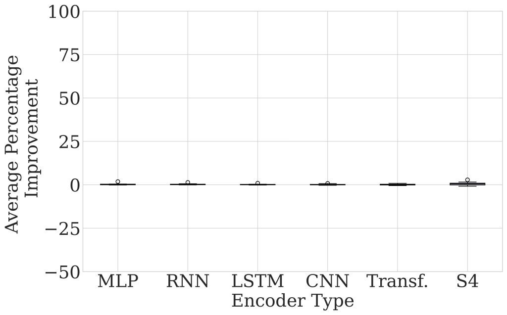
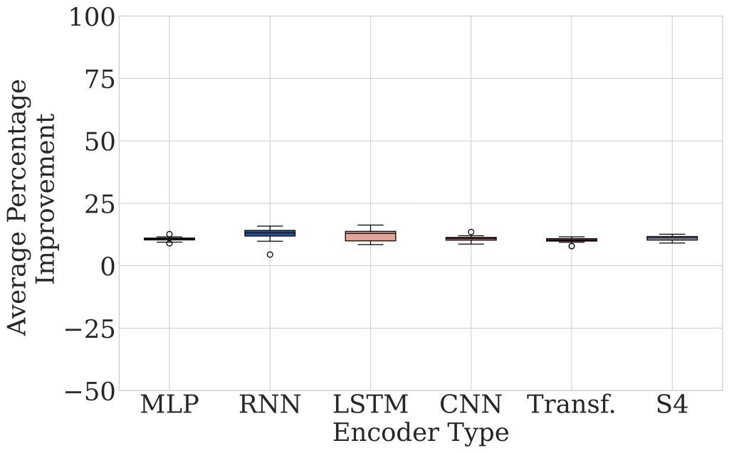
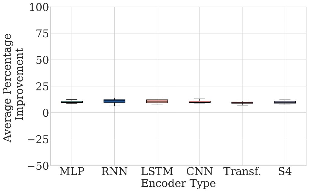
forking-sequences モデルにおいて、推論時にアンサンブル手法を適用することで、すべてのエンコーダーでアンサンブルなしの場合と比較して予測のばらつき(volatility)を低減できることを示します。具体的には、forking-sequences で訓練されたモデルに対して推論時に指数平滑化を適用すると、RNN、LSTM、CNN、Transformer、StateSpace ベースのアーキテクチャにおいて、それぞれ sEV の中央値パーセンテージ改善率が 13.2%、13.0%、10.9%、10.2%、11.2% 達成されます。これは、Fig. 5 に示すように sCRPS で 0.1% 未満の精度低下(劣化)しか生じないことを維持した上での結果です。
 image(a) sCRPS
 image(b) sEV
 image(c) sFPC
Fig. 5: forking-sequences 予測アンサンブルを適用した場合と適用しない場合の、異なるエンコーダータイプにおける各データセットでの (a) sCRPS、(b) sEV、(c) sFCP メトリクスの改善率分布。各データセットのメトリクスは 5 つのランダムシード実行の結果を平均化しています。改善率がゼロを超えることは、予測アンサンブルがより低い予測誤差またはばらつきを実現していることを示します。
さまざまなアンサンブル戦略(移動平均、移動中央値、累積平均、α = 0.1/0.5/0.9 の指数平滑化)を対象にアブレーション研究を実施した結果、高α(0.9)の指数平滑化が最もバランスの良い結果をもたらすことがわかりました。これは、より正確な短期予測に重みを置くことで、変動を平滑化する際の精度低下を最小限に抑えるためです。一方、α値を小さくすると変動はさらに抑制されますが、その分、精度へのコストが高くなります。
付録:事前学習済み基盤モデルにおけるゼロショットでの変動削減
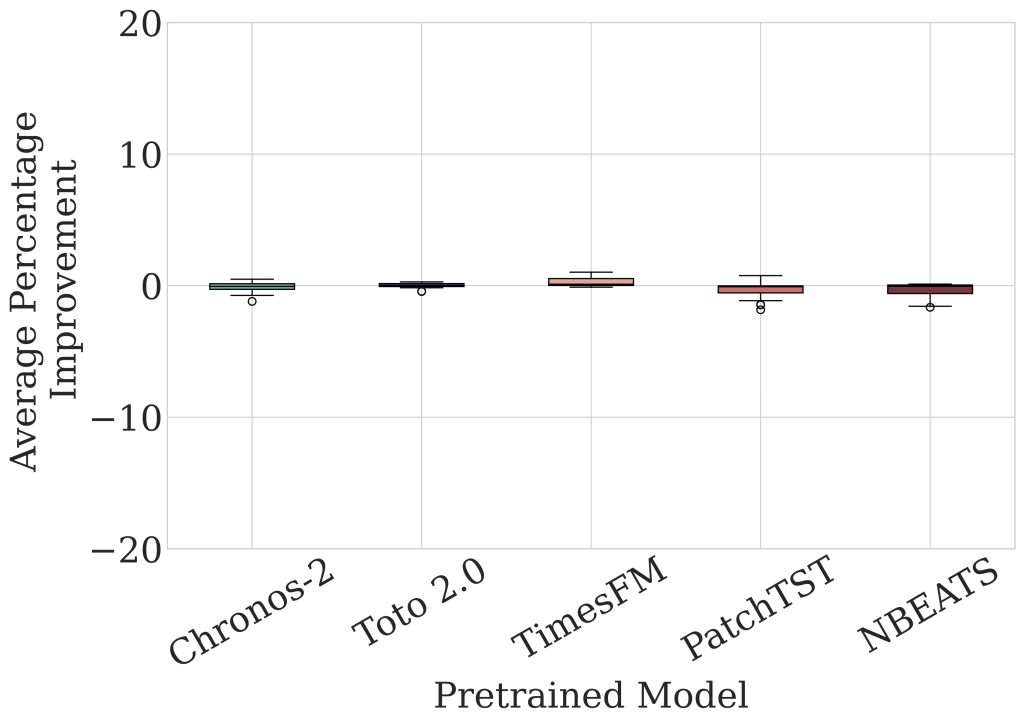
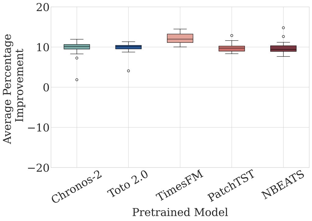
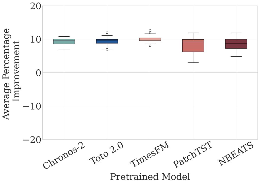
予測アンサンブルの恩恵は、フォークシーケンスを用いて特別に訓練されたモデルに限定されません。予測修正出力を収集することで、ウィンドウサンプリングで元々訓練された事前学習済みモデルにも予測アンサンブルを適用できます。ここでは、ゼロショット設定において、Chronos-2、Toto 2.0、TimesFM、および事前学習済み PatchTST と NBEATS を含む時系列基盤モデル(TSFMs)を用いてその実証を行います。
 image(a) sCRPS
 image(b) sEV
 image(c) sFPC
図 6: フォーキング・シーケンスによる予測アンサンブルと、アンサンブルなしを比較した際の、各データセットにおける (a) sCRPS、(b) sEV、(c) sFPC の改善率の分布。改善率がゼロを超えていることは、予測アンサンブルが予測誤差や変動性を低減できていることを示しています。予測アンサンブルは、予測精度(sCRPS)を維持しつつ、予測の変動性(sEV、sFPC)を大幅に低減できます。これは、フォークイング・シーケンスまたはウィンドウ・サンプリングのいずれで訓練されたモデルにも適用できる汎用的な推論技術としての有用性を示しています。
M シリーズベンチマーク全体を通じて、このシンプルな手法は予測変動性を中央値で約 10% 削減し、精度(sCRPS)への悪影響は 0.1% 未満に抑えました。つまり、フォークイング・シーケンス方式の集約による予測アンサンブルは、基盤モデルが元々フォークイング・シーケンスで訓練されたかどうかに関わらず、予測パイプラインに適用できる汎用的かつ実質的にコストのかからない技術です。

取りまとめ
1
Forking-sequences のグリッド構造は、自然に FCD 間で重複する予測を生成します。これにより、推論時に既に計算済みのエンコーダー出力を再利用することで、ほぼ無料のアンサンブルが可能になります。
2
新しいスケーリングされた過剰ボラティリティ(sEV)指標は、精度向上につながる修正と有害な修正を区別します。これは、単純な百分率変化に基づくボラティリティ測定法よりも実質的な改善です。
エンコーダーアーキテクチャの精度を犠牲にすることなく、指数平滑化を用いたフォークシーケンス予測のアンサンブルにより、変動性(volatility)は約10〜13%削減されます。
この恩恵は、Chronos-2、Toto 2.0、TimesFMといった事前学習済みファウンデーションモデルにおけるゼロショット利用にも及び、精度コストが0.1%未満で予測の変動性を約10%低減できます。
フォークシーチングでは、トレーニング時と推論時の両方でアンサンブルを統合可能であり、[2] で探求されたように学習可能なパラメータを用いてさらに拡張できることを認識しています。ただし、トレーニング時のアンサンブル統合については今後の課題とします。
本シリーズの第I部および第II部は、フォークシーケンスに関する理解を深め、オープンソースのニューラル予測ライブラリや将来の研究においてデフォルトのアーキテクチャオプションとして採用されるよう促すことを目的としています。また、この研究は標準的な精度指標に代わるものではなく補完するものとして変動性指標の重要性を強調し、その評価プロセスへの日常的な導入を呼びかけています。
参考文献:
[1] Rob J. Hyndman and Anne B. Koehler. Another look at measures of forecast accuracy. International Journal of Forecasting, 22(4):679 – 688, 2006. ISSN 0169-2070.
Carson Eisenach、Yagna Patel、Dhruv Madeka の「MQTransformer:文脈依存性とフィードバック認識型アテンションを用いたマルチホライズン予測」。Maria Florina Balcan と Marina Meila 編。第38回国際機械学習会議(ICML)プロシーディングスへの投稿。PMLR。作業版は arXiv:2009.14799 で公開されています(2021年8月)。
原文を表示
Based on: Potosnak, W., Wolff, M., Cao, M., Ma, R., Konstantinova, T., Efimov, D., Mahoney, M.W., Oreshkin, B., & Olivares, K.G. "Forking-Sequences: Statistically and Computationally Efficient Multi-Horizon Forecasting with Reduced Volatility." Transactions on Machine Learning Research, 2026.
(Disclaimer: Code implementation not used in the paper; not affiliated with Amazon — provided as a reference for forking-sequences and forecast ensembling)
TL;DR
Ensembling, nearly for free. Forking-sequences already produces overlapping forecasts for every target date across FCDs in a single forward pass, so ensembling them at inference adds no extra encoder computation compared with window-sampling.
Two new forecast volatility metrics. scaled Forecast Percentage Change (sFPC) measures raw revision size in real time (no ground truth needed); Excess Volatility (EV) goes further, rewarding accuracy-improving revisions and only penalizing the ones that move forecasts away from the truth or overshoot it.
Reduced volatility without sacrificing accuracy. Exponential-smoothing forecast ensembling (α = 0.9) reduces sEV by 10–13% across all encoder types, with less than 0.1% accuracy degradation.
Works zero-shot on models pretrained with window-sampling. Forecast ensembling applied to pretrained Time Series Foundation Models (TSFMs) — Chronos-2, Toto 2.0, TimesFM, PatchTST, N-BEATS — cuts volatility by ~10% with negligible accuracy cost (less than 0.1%).
In Part I, we introduced forking-sequences, a neural network architectural design that jointly encodes and decodes a time series across all forecast creation dates (FCDs) in a single forward pass. We showed why it's a statistically and computationally more efficient training paradigm than window-sampling. In Part II, we turn to a different but equally important problem: forecast volatility.
Why Forecast Volatility Matters
Accuracy is usually the headline metric for a forecasting model, but it isn't the only thing that matters in production. As a multi-horizon forecasting system operates over time, it generates multiple overlapping forecasts for the same future target date — one from each new FCD as more data becomes available. This sequence of updates is a forecast revision, and how consistent (or erratic) those revisions are is what we define as forecast volatility.
image(a) Without forecast inference ensembling
image(b) With forecast inference ensembling
Fig. 1: Forecasts (a) without and (b) with forecast ensembling applied. Forecast ensembling reduces volatility across FCDs, resulting in more stable and consistent forecast distributions. Red arrows indicate the direction of forecast revisions. Lines show P50 (median) forecasts across different FCDs. By reusing encoder computations, forking-sequences enables computationally efficient forecast ensembling with negligible additional cost.
Consider an electrical grid operator using load forecasts to plan power supply. If a forecast revises from 45 GW to 65 GW ahead of a heat wave, that's a useful revision; it tells operators to activate reserve plants. But if forecasts jump around erratically between FCDs without new information justifying the change, that undermines trust and complicates planning. The goal isn't to eliminate revisions, it's to distinguish benign, informative revisions from excessive, erratic ones.
This raises two questions we tackle directly in the paper:
?
How do we measure forecast volatility in a way that separates useful revisions from harmful ones?
?
Are there architectural designs that reduce volatility without hurting accuracy?
Forking-Sequences as a Natural Forecast Ensembling Mechanism
Because forking-sequences generates forecasts for every FCD in a single forward pass, it naturally produces multiple overlapping predictions for the same target date. Recall the forecast revision relationship: the prediction for a given target made at FCD t+1 is a revision of the prediction made at FCD t for the same date. Forecast revisions with the forking-sequences paradigm are shown in Fig. 2.
imageFig. 2: Forking-sequences
This overlapping grid structure means forking-sequences models can be ensembled for free (or nearly so) at inference time in terms of saving encoder computation compared with window-sampling, which requires multiple independent model forward passes. Given forecasts outputs via forking-sequences, we just average (or otherwise combine) the different FCD-level predictions for the same target date portrayed as the diagonal band in Fig. 3a:
\[
\begin{equation}
\widetilde{\mathbf{Y}}_{t,h} = \frac{1}{H}\sum_{k=0}^{H} \widehat{\mathbf{Y}}_{t-k, h+k} \qquad \text{for } t\geq H.
\label{eq:forking_sequences_ensemble}
\end{equation}
\]
image(a) Forking-sequences forecast ensemble
image(b) Forecast volatility reduction
Fig. 3: We adapt forking-sequences during inference to ensemble multiple forecasts of the same future date by computing a function (ex., moving average) across predictions generated from previous FCDs. b) Forking-sequences ensembling reduces forecast volatility, reducing the estimators variance with a linear convergence rate analogous to the weak law of large numbers.
Although it is tempting to expect a variance-reduction behavior similar to the results of Theorem 1, it is important to recognize that forecast variance naturally increases the further a forecast is from its corresponding observation. As a result, there is an inherent limit to how much ensembling can reduce volatility: older forecast revisions carry substantially higher uncertainty, whereas more recent revisions are both more accurate and less variable. This makes it desirable for an ensemble to place greater weight on newer forecasts rather than treating all revisions equally.
New Forecast Volatility Metrics
We introduce scaled Forecast percentage Change (sFPC) to measure the relative change in predicted quantiles across consecutive forecast creation dates, providing a quantitative view of temporal volatility or forecast revision rates. Inspired by the sMAPE metric, sFPC uses a symmetric denominator, based on both current and previous forecasts, to mitigate issues of numerical instability [1]. This design ensures robustness when dealing with small predicted values and avoids the division-by-zero problems common in traditional percentage-based metrics.
\[
\mathrm{sFPC}^{(q)}\left(\hat{\mathbf{y}}^{(q)}_{[b][t][h]}\right)
= \frac{200}{B \times T \times H} \sum_{b,t,h} \frac{|\hat{y}^{(q)}_{b,t+1,h}-\hat{y}^{(q)}_{b,t,h+1}|}{|\hat{y}^{(q)}_{b,t+1,h}| + |\hat{y}^{(q)}_{b,t,h+1}|} .
\]
Computing sFPC between consecutive forecasts treats all revisions as equally undesirable, even ones that clearly improve accuracy. To address this, we also introduce scaled Excess Volatility (sEV), a metric for probabilistic forecasts that only penalizes revisions that move a forecast away from the truth, or that overshoot it. sEV is designed to reward accuracy-improving forecast revisions while distinguishing them from harmful volatility. sEV is defined as:
\[
\mathrm{sEV}\left(\mathbf{y}_{[b][t][h]}, \hat{\mathbf{y}}_{[b][t][h]}\right) = \frac{\sum_{b,t,h} \mathrm{EV}(y_{b,t,h}, \mathbf{\hat{y}}_{b,t,h+1}, \mathbf{\hat{y}}_{b,t+1,h})}{\sum_{b,t,h} |y_{b,t,h}|}, \quad \text{where}
\]
\[
\mathrm{EV}(y,\;\mathbf{\hat{y}}_1,\; \mathbf{\hat{y}}_2) = \mathrm{QL}(\mathbf{\hat{y}}_2,\mathbf{\hat{y}}_1) - (\mathrm{QL}(y,\mathbf{\hat{y}}_1)-\mathrm{QL}(y,\mathbf{\hat{y}}_2)), \quad \text{and}
\]
\[
\mathrm{QL}_q(y, \hat{y}^{(q)}) = q(y-\hat{y}^{(q)})_+ + (1-q)(\hat{y}^{(q)}-y)_+ .
\]
EV has three useful properties, proven formally in the paper:
Zero penalty for improving revisions, shown in Fig. 4a: if a revision moves proportionally closer to the ground truth, landing on the direct path between the truth and the prior forecast, EV = 0.
Maximum penalty for deteriorating revisions, shown in Fig. 4b: if a revision moves the forecast further from the truth, with the old forecast sitting between the truth and the new one, EV equals the full accuracy degradation, the difference in quantile loss between the new forecast and the old one.
Overshoot penalty, shown in Fig. 4c: if a revision moves in the right direction but overshoots, with the truth landing between the old and new forecast, EV penalizes only the new forecast's quantile loss against the truth.
image(a) Improving revision
image(b) Deteriorating revision
image(c) Overshooting revision
Fig. 4: Example penalty behavior of the Excess Volatility (EV) metric. EV distinguishes accuracy-improving revisions from accuracy-degrading ones, assigning no penalty when revisions improve accuracy, while asymmetrically penalizing both deteriorating and overshooting revisions according to their impact on accuracy.
One important distinction: sFPC can be computed at prediction time for real-time monitoring, since it doesn't require ground truth. sEV, by contrast, depends on the ground-truth value, so it can only be applied retroactively to assess forecast volatility.
Empirical Results: Volatility Reduction Without Sacrificing Accuracy
The core empirical claim: for forking-sequences models, applying exponential-smoothing ensembling at inference (α = 0.9) reduces forecast volatility (sEV) substantially while maintaining forecast accuracy.
We show that for forking-sequences models, forecast ensembling during inference can reduce forecast volatility compared to forecasts without ensembling for all encoders. Specifically, applying exponential smoothing at inference to models trained with forking-sequences yields median percentage improvements in sEV across datasets of 13.2%, 13.0%, 10.9%, 10.2%, and 11.2% for RNN, LSTM, CNN, Transformer, and StateSpace-based architectures, respectively, while maintaining forecast accuracy (less than 0.1% degradation in sCRPS as shown in Fig. 5).
image(a) sCRPS
image(b) sEV
image(c) sFPC
Fig. 5: Distribution of percentage improvement in (a) sCRPS, (b) sEV, and (c) sFPC metrics across datasets for different encoder types with forking-sequences forecast ensembling compared with no ensembling. Each dataset's metric is averaged over 5 random seed runs. Percentage improvement greater than zero indicates forecast ensembling achieves lower forecast error or volatility.
We include an ablation study across different ensembling strategies (moving average, moving median, cumulative average, exponential smoothing at α = 0.1/0.5/0.9), and find that exponential smoothing with high α (0.9) gives the best trade-off; it weights near-term (more accurate) forecasts more heavily, minimizing the accuracy cost of smoothing out volatility. Lower α values reduce volatility further but at a higher cost to accuracy.
A Bonus: Zero-Shot Volatility Reductions for Pretrained Foundation Models
Forecast ensembling benefit isn't limited to models specifically trained with forking-sequences. We can apply forecast ensembling to pretrained models originally trained with window-sampling by collecting forecast revision outputs. We demonstrate this with pretrained Time Series Foundation Models (TSFMs), including Chronos-2, Toto 2.0, TimesFM, and pretrained PatchTST and NBEATS, in a zero-shot setting.
image(a) sCRPS
image(b) sEV
image(c) sFPC
Fig. 6: Distribution of percentage improvement in (a) sCRPS, (b) sEV, and (c) sFPC metrics across datasets for different encoder types with forking-sequences forecast ensembling compared with no ensembling. Percentage improvement greater than zero indicates forecast ensembling achieves lower forecast error or volatility. Forecast ensembling can substantially reduce forecast volatility (sEV, sFPC) while maintaining forecast accuracy (sCRPS), demonstrating its utility as a general-purpose inference technique for models trained with either forking-sequences or window-sampling.
Across the M-series benchmark, this simple technique achieved a median ~10% reduction in forecast volatility, with less than 0.1% degradation in accuracy (sCRPS). In other words: forecast ensembling via forking-sequences-style aggregation is a general-purpose, nearly-free technique that can be used in forecasting pipelines regardless of whether the underlying model was originally trained with forking-sequences.
image Takeaways
1
Forking-sequences' grid structure naturally produces overlapping forecasts across FCDs, enabling near-free ensembling at inference time by reusing already-computed encoder outputs.
2
The new scaled Excess Volatility (sEV) metric distinguishes accuracy-improving revisions from harmful ones — a meaningful improvement over naive percentage-change volatility measures.
3
Ensembling forking-sequences forecasts via exponential smoothing cuts volatility by ~10–13% across encoder architectures without sacrificing accuracy.
4
This benefit extends to zero-shot use with pretrained foundation models like Chronos-2, Toto 2.0, and TimesFM, achieving approximately 10% reduced forecast volatility with <0.1% accuracy cost.
We acknowledge that ensembling can be integrated during both training and inference with forking-sequences, and could be further extended with learnable parameters as explored in [2]. We leave training-time ensembling integration to future work.
Together, Parts I and II aim to build broader awareness of forking-sequences and promote its adoption as a default architectural option in open-source neural forecasting libraries and future research. This work also advocates for greater awareness of volatility metrics as a complement to standard accuracy metrics, encouraging their routine adoption in forecasting evaluation.
References:
[1] Rob J. Hyndman and Anne B. Koehler. Another look at measures of forecast accuracy. International Journal of Forecasting, 22(4):679 – 688, 2006. ISSN 0169-2070.
[2] Carson Eisenach, Yagna Patel, and Dhruv Madeka. MQTransformer: Multi-Horizon Forecasts with Context Dependent and Feedback-Aware Attention. In Maria Florina Balcan and Marina Meila, editors, Submitted to Proceedings of the 38th International Conference on Machine Learning. PMLR. Working Paper version available at arXiv:2009.14799, 8 2021.
関連記事
今日のまとめ
AIデイリーブリーフで今日の重要ニュースをまとめ読み