Claude の生成テキストに埋め込むウォーターマークの仕組みを解説
本文の状態
日本語全文を表示中
詳細モードで約17分の本文を読めます。
同じ出来事の情報源
この情報源を基点に整理
Sebastian Raschka
Sebastian Raschka は Anthropic が Claude モデルの出力テキストに導入する新しいウォーターマーキング技術の詳細解説動画を公開し、その仕組みや限界について分析している。
AI深層分析を開く2026年8月22日 20:26
AI深層分析
キーポイント
詳細解説動画の公開
Sebastian Raschka は Anthropic の発表を受けて、従来の記事形式ではなく、52スライド・48分間の講義動画を制作して技術的詳細を解説した。
ウォーターマーキングの仕組みと限界
動画ではテキストウォーターマーキングがどのように機能するかを説明し、同時にこの手法が失敗したり除去されたりする可能性についても言及している。
技術的メリットと懸念の分析
LLM 生成テキストへのウォーターマーキング導入は、テキスト品質を低下させるという懸念がある一方で、その実装方法や利点を理解することで判断材料を提供する。
ゼロから実装する価値
LLM をゼロからコーディングすることで、サンプリング内部の実装やウォーターマークの適用位置など、抽象化された層に隠れた詳細を深く理解できる。
コード読解の重要性
LLM によるコーディングが一般的になった現在でも、コードを読むことは多くの情報を伝達するため依然として有用である。
重要な引用
Anthropic announced that they will watermark the text outputs of their Claude models.
I think if we understand a bit better what watermarking is, that goes a long way, and then we can make up our own minds about whether that's a good thing or not.
"coding from scratch is actually a very, very useful technique because it really helps you understand how something is implemented."
"it is still useful being able to... build something from scratch for educational purposes to understand something deeply and then also for research purposes to manipulate this in a transparent way that is not hidden away in tons of layers of abstraction."
編集コメントを表示
編集コメント
Sebastian Raschka のような技術アナリストによる詳細な解説動画は、単なる発表内容を超えて実装の裏側やリスクを可視化する点で価値が高い。業界関係者は、この技術が実際の運用環境でどのように機能し、どのようなバイアスや脆弱性を生むかを注視する必要がある。
Source Article
元記事を日本語で読む
本文に関係しない購読案内、埋め込み通知、サイト内プロモーションは除いています。
最近、Claude の新しいテキストウォーターマーキングのプロセスと実装について Substack で投稿しました。この話題が非常に人気を集め、活発な議論を巻き起こしたため、仕組みの詳細をもう少し掘り下げて説明してみようと思いました。
いつもの記事形式ではなく、今回は少し趣向を変えて、このテーマに関する短い講義動画を撮影しました。以下に動画と、その文字起こしを掲載します。
当初はスライド 10 枚程度で 10 分ほどの短編動画を想定していましたが、構成を進める中で重要な詳細情報をいくつか追加した結果、最終的には 50 枚を超えるスライドと 48 分の動画となりました。
これで仕組みがより明確に理解いただけたことを願っています。ぜひご覧ください!
YouTube プレーヤーを利用したい場合は、YouTube 版も用意しています。
また、スライドへのリンクはこちらです。
購読はこちらから
動画文字起こし
※以下の文字起こしは可読性を高めるために一部編集・整理されていますが、上記の講義動画全体の順序と流れは保持されています。
0:00
Claude のテキストウォーターマーキングの仕組み
スライド 2/52(時刻:0:00)
こんにちは。数日前、Anthropic が Claude モデルのテキスト出力にウォーターマークを埋め込むと発表しました。私は直後にソーシャルメディアでその仕組みについて簡潔な解説を投稿したのですが、これが非常に反響を呼びました。
注目されたのはウォーターマーク自体というより、その仕組みや背景にある技術についての説明だったようです。そこで今回は、単一の図だけでは不十分だったため、もう少し詳しく解説する価値があると考え、記事にしました。元々はスライド 10 枚程度で解説しようと考えていたのですが、最終的には 50 枚の図解を用意することになりました。
この技術がどのように機能するのか、またウォーターマークがなぜ失敗したり削除されたりするのかといった点についても詳しく説明できればと思います。最近では多くの人が LLM を利用しており、インターネット上で生成されたテキストも増えています。そのため、この話題は興味深いものになるでしょう。
さて、今回のウォーターマーク化について、「テキストの質が低下するのではないか」という懸念や、果たしてどのようなメリットがあるのかという疑問も出ています。しかし、ウォーターマークとは何かを正しく理解できれば、その是非や長所・短所について自分たちで判断できるようになります。
今回の目的は、Claude が生成したテキストに埋め込むウォーターマークの仕組みと、その実装方法について解説することです。
スライド 2/52(タイムスタンプ 1:41)
このウォーターマーク技術は、従来のモデルや大規模言語モデル(LLM)が内部でどのように動作しているかを理解する絶好の例でもあります。私は「ゼロから作る」アプローチを好むので、こうした解説もその一環です。
私の著書『Build a Large Language Model From Scratch』や『Build a Reasoning Model From Scratch』、『From Scratch』シリーズの記事などでも、この考え方を貫いています。
私にとって「ゼロから作る」とは、コードを書くことを意味することが多いです。今回の解説ではコーディングは行いませんが、「ゼロから実装する」ことは非常に有益な手法です。なぜなら、仕組みを深く理解するためには、実際にコードを書いてみるのが一番だからです。実装を通じて初めて、数式や概念、図解の意味が明確になります。コードがないと、説明が曖昧になりがちなのです。
もちろん、誰もがゼロからコーディングする時代ではなくなったことも事実です。
昔は、ゼロからコードを書くことこそが唯一の手段でした。つまり、プログラムを組めるのは人間だけだったのです。現在は LLM(大規模言語モデル)によるコーディングも可能になりました。しかし、コードを読む価値がなくなるわけではありません。コードには多くの情報が詰まっているからです。
この文脈で言えば、LLM をゼロから実装するために時間をかけることは、内部のサンプリング処理がどのように実装されているかを理解する上で非常に役立ちます。関連するコードスニペットもいくつか残っています。
その結果、ウォータマーキング(透かし)がどこに適用され、どのような影響があるのかを深く理解できるようになります。人々が必ずしもゼロからコーディングしているわけではないとしても、教育目的で何かをゼロから構築し、本質を深く理解したり、研究のために抽象化の層に隠されることなく透明性を持って操作したりする能力は依然として有用です。
さて、それはともかく、このスライド資料では私の「ゼロから作る」教材から多くの図を使用しているため、結果的に良い関係性が生まれたのだと思います。
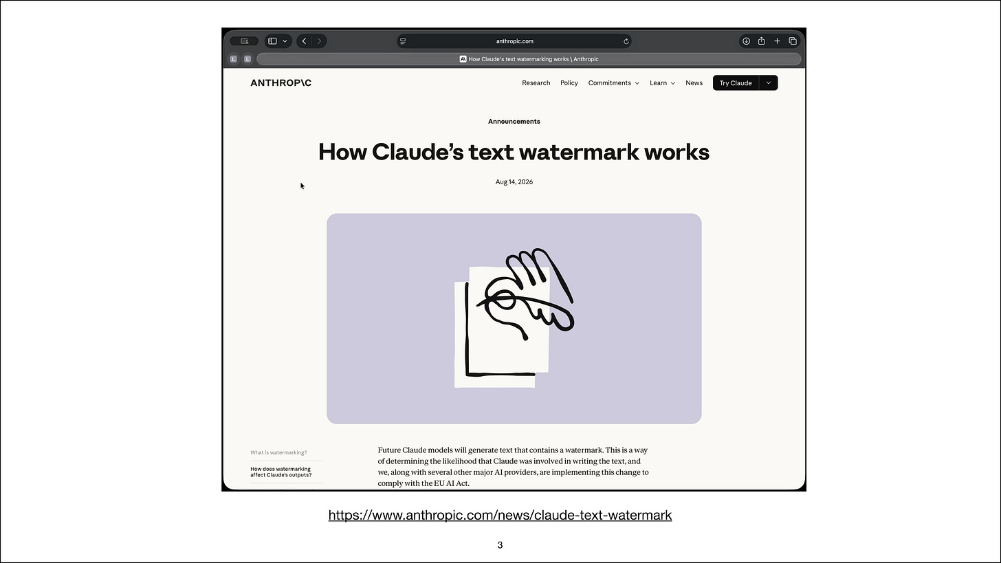
スライド 3/52、タイムスタンプ 3:58
先日(8 月 14 日時点)、「Claude のテキストウォーターマークの仕組み」や、スライドの内容をすべて収録したスクリーンレコーディング動画が公開されました。実はこの情報は数回更新されており、私が最初に読んだときはもっと簡潔な内容でした。
しかし、全体的に概念的な説明が多く、図解は一つもありません。そのため、「彼らが何を実現しようとしているのか」を直感的に理解するのはまだ難しいのが実情です。なぜその手法を採用するのかという動機については詳しく説明されていますが、具体的な「どのように行うか」というプロセスには触れられていません。関連する論文へのリンクも存在しますが、こちらは非常に技術的な内容です。
そこで、このウォーターマーク技術をどう実装しようとしているのかを理解するために、一度立ち止まって基本から振り返ってみることにしましょう。
まず、ウォーターマーク化の目的は、誰かが公開したテキストが「Claude Opus 4.8 モデル」によって生成されたものかどうかを特定できることです。これにより、「このテキストには AI 特有のウォーターマークが含まれているため、AI 生成物である」と判断する根拠となります。ただし、このウォーターマークは一般ユーザーには見えないように設計されており、デコードして存在を確認できるのは開発者側だけです。
なぜ開発者だけがそれができるのかについては、後ほど詳しく解説します(動画が長くなりすぎないよう努めます)。まずは一歩ずつ進んでいきましょう。
5:38
LLM によるテキスト生成の仕組み
スライド 4/52、タイムスタンプ 5:35
まず、テキスト生成がどのように行われるのかを簡単に説明し、その上でウォータマーキングの仕組みを理解していただきたいと思います。これにより、この技術が追加コストのかかる大掛かりなものではなく、通常のテキスト生成プロセスに施されるごく小さな調整に過ぎないことがお分かりいただけるはずです。
スライド 5/52、タイムスタンプ 6:01
例えば ChatGPT を使っているときを想像してください。「ドイツの首都は?」と質問すると、ChatGPT や他の大規模言語モデル(LLM)は「ベルリン」と答えます。この場合、「ベルリン」とピリオドという 2 つのトークンを生成しています。ただし説明を簡単にするため、ここでは 1 つのトークンが生成されると仮定しましょう。つまり、次のトークンは「ベルリン」です。
では、内部ではどのようにしてこのトークンが生成されているのでしょうか?
「ドイツの首都は」と入力して「ベルリン」というトークンを受け取ったとき、裏側でいったい何が起きているのでしょうか?
スライド 6/52、タイムスタンプ 6:41
次の数枚のスライドでは、次に生成されるトークンが裏側でどのように処理されているのかを簡単に解説します。
スライド 7/52、タイムスタンプ 6:50
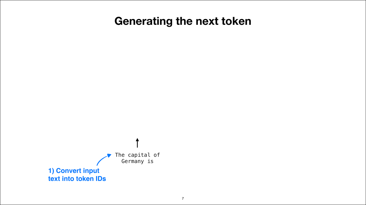
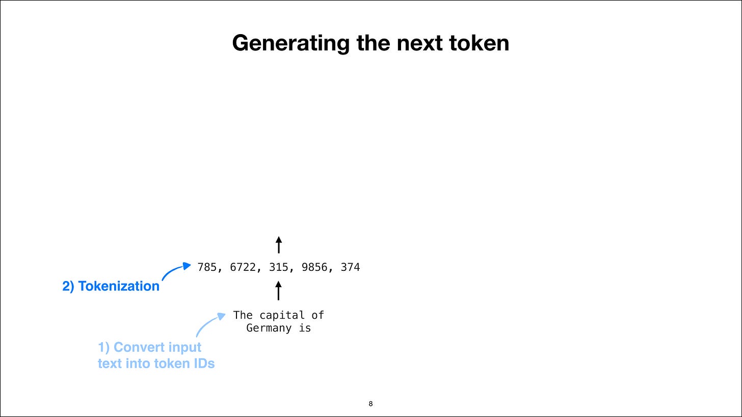
ここでは、プロンプトを「ドイツの首都は」と仮定して話を進めます。まず行うべきステップは、これをトークン ID に変換することです。テキストをトークン化し、ID に変換する処理は、初期段階における主要な工程の一つです。
この処理は LLM(大規模言語モデル)の外側で行われるものであり、LLM の内部プロセスではありません。つまり、単にテキストを LLM が扱える形式であるトークン ID へ変換しているだけです。
スライド 8/52、タイムスタンプ 7:22
その後、データは LLM を通過し、LLM が次のトークンに対するスコア分布を出力します。
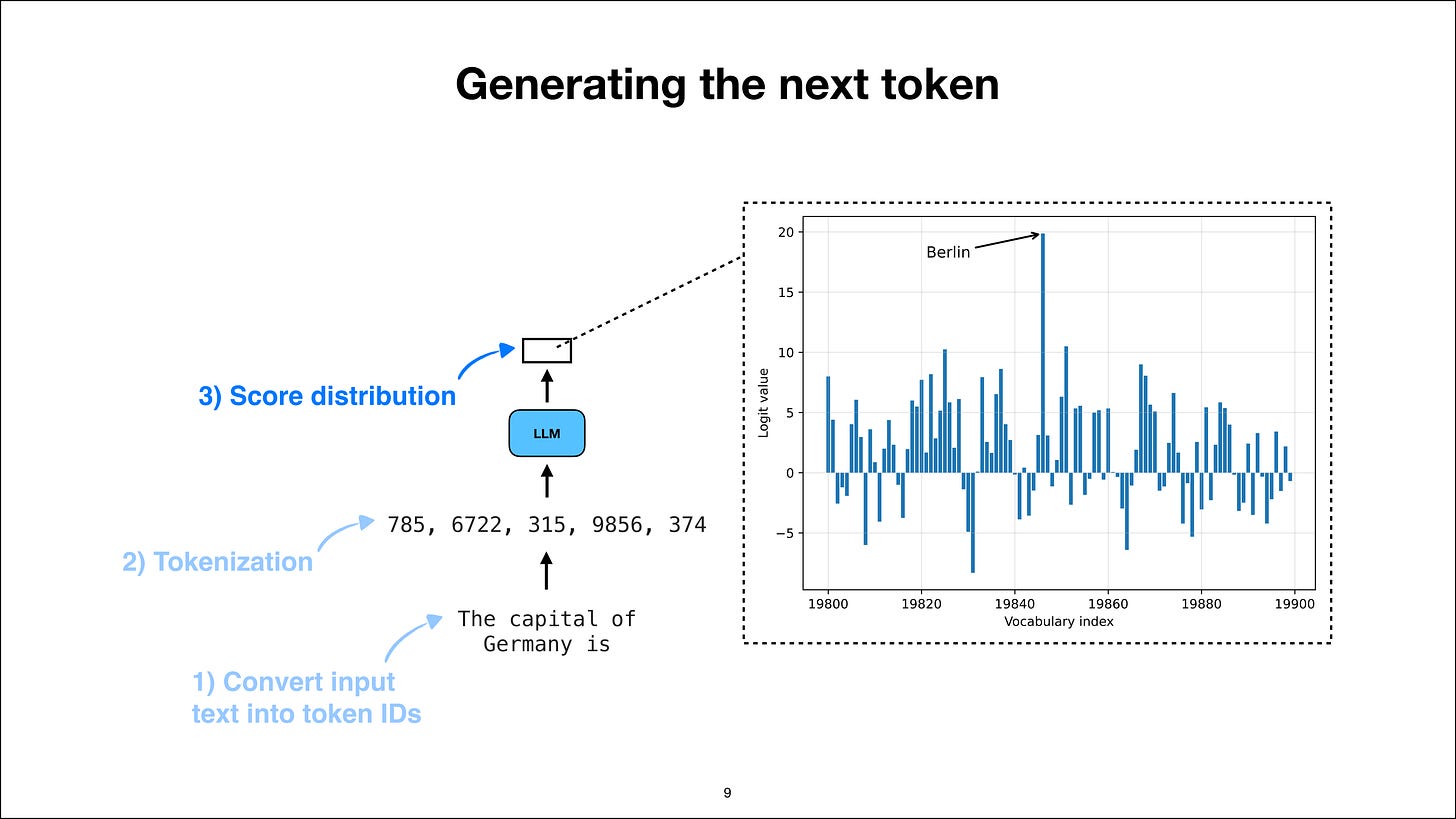
スライド 9/52、タイムスタンプ 7:31
改めて、大規模言語モデル(LLM)の内部動作を簡単に振り返っておきましょう。ここでは LLM の仕組みそのものについては深く掘り下げません。私の他の「ゼロから作る LLM」シリーズの動画や書籍で何度も解説している通りです。
重要なのは、次のトークン(例えば「Berlin」)を生成する際、この時点でスコアの分布が存在している点です。これが LLM が出力した結果となります。
今回のケースでは、ロジット値を見ています。これはマイナス無限大からプラス無限大までの範囲にあるスコアそのものです。具体的には、約 -8 または -9 から 20 程度の範囲の値が並んでいます。
これらの値を確率分布に変換することも可能ですが、サンプリングの方法によっては厳密に必要とは限りません。つまり、ロジット値は「生のスコア」として捉えておけばよいのです。
この生のスコアは、すべての語彙(ボキャブラリ)に対して計算されます。
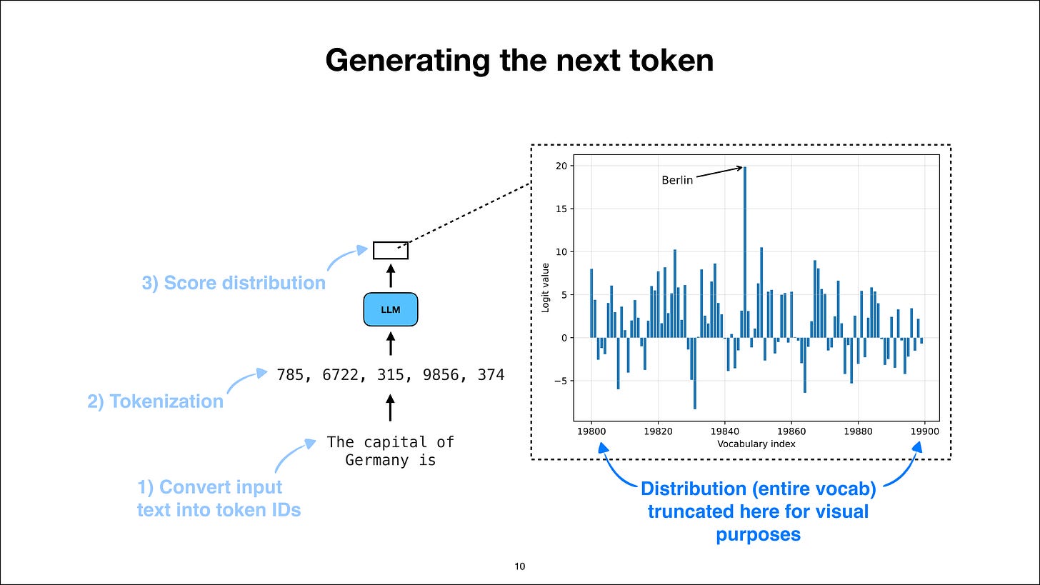
スライド 10/52、タイムスタンプ 8:39
つまり、LLM が生成しうるすべての単語が対象となります。ここで注目すべきは語彙インデックスです。特定の値(インデックス位置 19,846)が最も高いスコアを獲得しています。このため、私は分布を広げて表示しています。
もしこのプロンプトを LLM に実行させると、さらに極端な結果が見られるはずです。つまり、すべての値がほぼゼロに近い状態になるでしょう。その中で「Berlin」のスコアは、他の単語に比べて格段に高くなるはずです。
ただ、いくつかのピーク(山)を見せることで、少し興味深い見た目にするために、私はこの部分を拡大表示し、分布を広げています。ここで「Berlin」が最高スコアとなっているのは、このような具体的なプロンプトに対して、それが最も確からしい次のトークンであると考えることができるからです。他の単語については、例えば「Hamburg」や「Munich」のように、LLM が誤って推測する可能性のあるものも含まれます。
しかし現在では、LLM はここで正解が「Berlin」であることをかなり確信しているはずです。また、ここに表示されているのは語彙インデックスです。これは全体の語彙にわたるものです。現在の LLM では、出力可能なトークンが約 250,000 種類あります。
このスライドではスペースの都合上、19,800 から 19,900 の範囲に切り詰めて表示しています。もし現実的な 250,000 単語の語彙をそのまま表示すると、分布があまりにも細くなりすぎて、このグラフ上でほとんど何も識別できなくなるでしょう。
これは教育目的のために一部省略した内容です。重要な点は、通常のテキスト生成ではこのようなスコア分布が得られることです。次に、私たちはこの中で最も高いスコアに注目します。
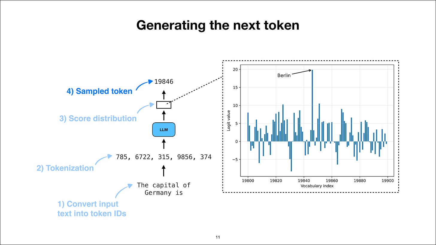
スライド 11/52、タイムスタンプ 10:33
この選択がどのように行われるかについては後ほど詳しく説明しますが、必ずしも厳密に最高スコアを選んでいるわけではありません。ここでは簡略化のため、最も高いスコアを採用していると仮定してください。この場合の値は 19,846 です。
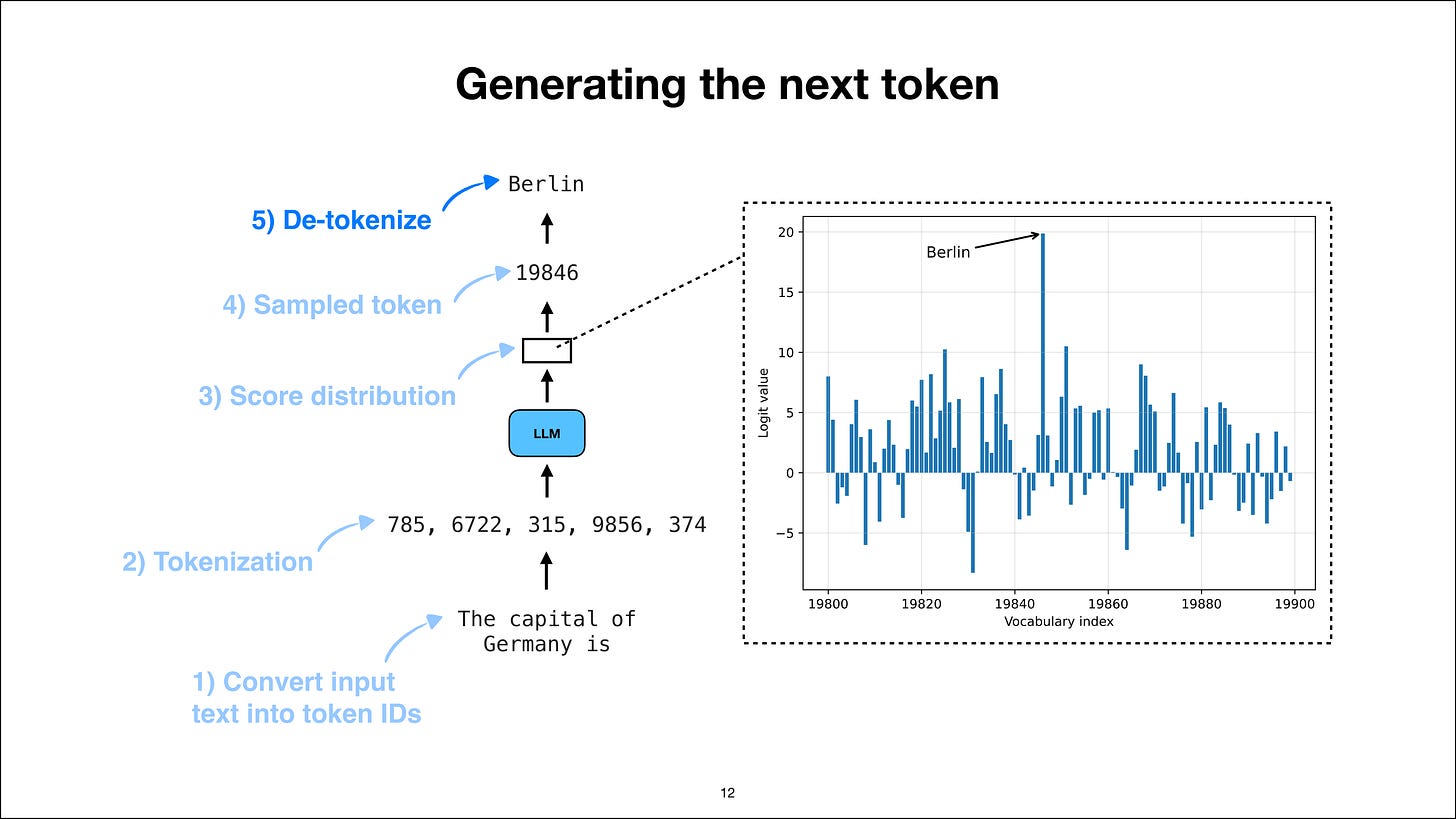
スライド 12/52、タイムスタンプ 10:52
このスコアはその後デトークン化され、「Berlin」という単語が復元されます。つまり、このスライドで示されているプロセスは以下の通りです。入力プロンプトからトークン ID への変換とトークナイゼーションを行い、LLM(大規模言語モデル)に渡してスコア分布を取得し、次のトークンを決定、最後にそれをテキストに戻すという一連の流れです。
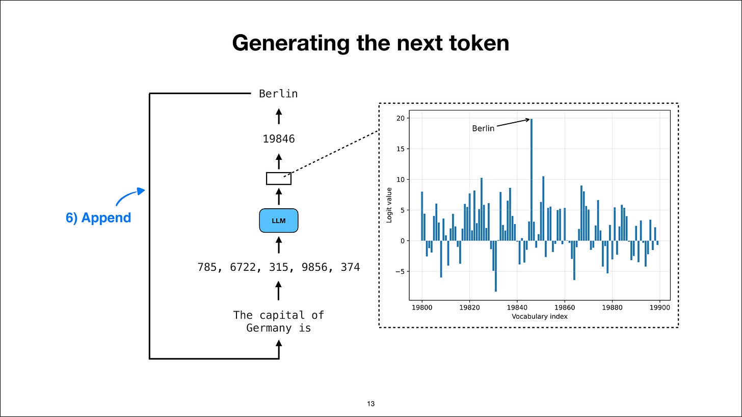
スライド 13/52、タイムスタンプ 11:12
そして、このテキストが入力に追加されます。したがって、複数のトークンを出力する必要がある質問に対しては、回答が完成するまでこのループを続けます。通常、LLM は「テキスト終了」トークンを生成することでこれを示します(例えば、ここ)。簡略化のため、ここでは 1 トークン生成の 1 回の反復のみを示していますが、前述した通り、修正された入力を LLM にフィードバックして次のラウンドへ続けるという流れになります。
では、実際にこの次のトークンをどのようにサンプリングするのでしょうか?
次のトークンサンプリングの仕組み
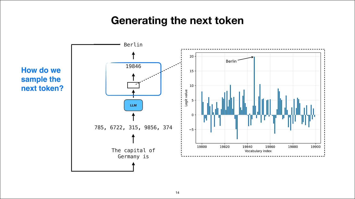
スライド 14/52、タイムスタンプ 11:44
少し触れましたが、技術的にはスコアが最も高いものを選ぶことも可能です。これを「貪欲デコーディング(greedy decoding)」と呼びます。確かにこの方法も存在しますが、実際に LLM を使う場合、常にスコアが最も高いトークンを選択する貪欲デコーディングは行われません。
なぜなら、別のプロンプトで質問された際に、常に最高スコアのものを選ぶと、モデルが学習データを単に暗記してしまいかねないからです。
同じような応答を繰り返し返すだけでは、出力に変化が生まれません。しかし、あまりにもランダムな内容になってしまっては困ります。では、どのようにしてこのバランスを保つのでしょうか?
まず、この分布からサンプリングする際、通常は確率スコアに変換します。
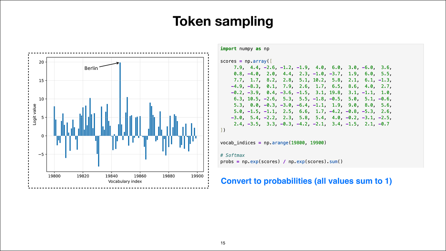
スライド 15/52、タイムスタンプ 12:28
ここでは、これらのスコアをプロットに表示しています。説明の便宜上 NumPy を使用していますが、PyTorch など他のツールを使用しても同じ概念が適用されます。仮に、NumPy でこれらのスコアを取得できたとしましょう。
次に私が行うのは、ソフトマックス(softmax)関数の計算です。実際には Torch や PyTorch などで実装された数値的に安定した softmax 関数を用います。これは、非常に大きな正の値や負の値、あるいはその逆のような極端な値に対しても正確に動作するものです。
ここでは可読性を高めるため、あえて簡略化して記述しています。細かい実装の詳細はここでは重要ではありません。
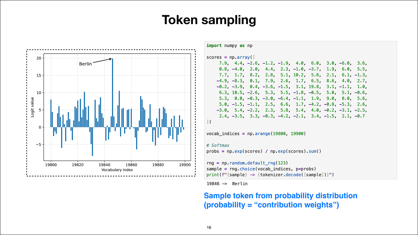
スライド 16/52、タイムスタンプ 13:20
重要なのは、この変換後におけるスコアです。スライドには表示できるスペースに限界がありますが、これらのスコアの合計は必ず1になります。つまり、これは本質的に再正規化(renormalization)であり、確率に変換する softmax 処理によって合計が1に収束します。
こうして得られた確率を用いれば、乱数やサンプリングアルゴリズムを利用して次のトークンを決定できます。例えば NumPy では choice 関数またはメソッドを使用します。ここでは特定の乱数シードを語彙インデックスに渡すことで再現性を確保し、さらに重要な点として、確率値を重み(weights)として指定します。
これはつまり、「あるトークンが選択される可能性はどれくらいか?」という問いに対する答えです。例えば、正規化ステップ、具体的には softmax 処理の後、「Berlin」の確率が99%で、他のすべてのトークンの確率の合計が1%しかない場合、100回サンプリングを行えば約99回は「Berlin」が選択されることになります。
例えば、よく訓練された現実的な大規模言語モデル(LLM)では、「Berlin」という単語に 99.999999% という確率が付与されるようなケースがあります。この場合、モデルが「Berlin」が正解であると非常に高い自信を持っているため、サンプリング結果はほぼ確実に「Berlin」になります。これが、この分布からサンプリングを行う基本的な仕組みです。
ただし、top-k サンプリングや top-p サンプリングといった改良手法も存在します。例えば top-k サンプリングでは、単純化のために上位 100 トークンを選別し、ランダム選択をその上位 100 トークンのみに適用します。これにより、意味のないトークンが混入するのを防ぎます。
今回の例では、この詳細は本質的に重要ではありません。あくまで説明のための追加要素に過ぎないため、ここでは簡潔に触れるにとどめます。したがって、すでに top-k などの手法によって上位 100 トークンに絞られた状態であると仮定して進めても問題ありません。
スライド 17/52(タイムスタンプ:15:37)
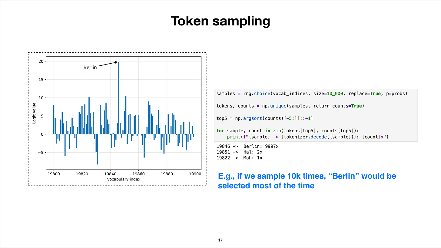
例えば、確率を「ベルリン」が非常に高い 99.9% に設定して 10,000 回サンプリングすると、「ベルリン」は 9,997 回、「Hal」が 2 回、「Moh」が 1 回出現します。これらは本質的に意味をなさないトークンです。
通常、LLM がこのような無意味な単語を生成することは稀ですが、今回はより興味深い例を示すために、あえて分布を広げています。
実際の LLM では、「ベルリン」の確率が極めて高いため、10,000 回サンプリングすればほぼ確実に「ベルリン」が出力されるはずです。ただし、これは説明のための例に過ぎません。
サンプリングからウォーターマーキングへ
スライド 18/52(時刻 16:21)
LLM の内部動作については、以前にも何度か解説してきましたが、今回はウォーターマーキングの仕組みを理解してもらうための文脈として、簡単に触れておきます。この概念自体も興味深いものです。
. So, below is the video along with a transcript.
Originally, I planned to make 10 slides and record a short 10-min video. However, while putting it together, I added some crucial details here and there, resulting in >50 slides and a 48 min recording.
I hope that this now explains it well, though! Happy watching!
I also have a YouTube version if you prefer using the YouTube player.
And here is a link to the slides
Subscribe now
Video Transcript
Note: The transcript below is slightly edited and cleaned up for readability but preserves the overall order and flow of the video lecture above.
0:00
How Claude’s Text Watermarking Works
Slide 2 of 52, time stamp 0:00
Hi everyone. So, a few days ago, Anthropic announced that they will watermark the text outputs of their Claude models. I then did a social media post briefly explaining how that works. And yeah, this was quite the popular post. So not the watermarking itself was popular, but I guess the explanation or the mechanism behind it. Then, it might be worthwhile expanding this a bit to explain it in more detail, because this post only had one figure, and there were a lot of questions and discussions.
So, I thought, well, let’s make a few more figures. I actually originally planned to do like 10 slides and walk you through it. It ended up being 50 slides, but I hope this really explains how this watermarking technique works well, how watermarking itself can fail or be removed, and so forth. So I think it might be an interesting topic because a lot of people use LLMs these days and also consume a lot of text on the Internet that might be generated by LLMs.
And now there’s going to be this watermarking, and there’s this, I guess, fear of watermarking making text worse, or what’s actually the benefit of this watermarking? And so what does it mean? And I think if we understand a bit better what watermarking is, that goes a long way, and then we can make up our own minds about whether that’s a good thing or not, and so forth, like the pros and cons.
So, my goal here is really to explain how the underlying mechanism works and how they are going to implement this type of watermarking, text watermarking.
Slide 2 of 52, time stamp 1:41
It’s also a great example to illustrate why understanding things from scratch is actually quite useful. This watermarking technique is also a nice way to explain how conventional models or LLMs in general work under the hood. So yeah, you may know I like doing things from scratch. Like, I have my books: Build a Large Language Model From Scratch, Build a Reasoning Model From Scratch. I have some articles labeled from scratch.
So, for me, “ from scratch often includes coding. So this one will not be coding-related, but coding from scratch is actually a very, very useful technique because it really helps you understand how something is implemented. And then from that we can derive our understanding, figures, concepts, because if we don’t really implement things, if there’s no code, it’s really sometimes ambiguous. And of course, you know, as I realized, not everyone is coding from scratch anymore.
Like back in the day, coding something from scratch was all we had. I mean, there were only humans coding. Nowadays, coding can be done by LLMs. However, that doesn’t mean reading code is no longer useful, because it carries a lot of information. So in this case here with this watermarking, spending some time coding an LLM from scratch really makes you realize how this sampling inside is implemented. We still have some relevant code snippets.
And then that really, in turn, helps us understand, oh, the watermarking is applied at this position, and this has so-and-so consequences and so forth. So I think even though people may not be coding from scratch, at least not all the time anymore, it is still useful being able to, let’s say, build something from scratch for educational purposes to understand something deeply and then also for research purposes to manipulate this in a transparent way that is not hidden away in tons of layers of abstraction.
But that aside, I think it’s just a coincidental nice relationship here because, for this slide deck, I actually used a lot of figures from my from-scratch coding materials.
Slide 3 of 52, time stamp 3:58
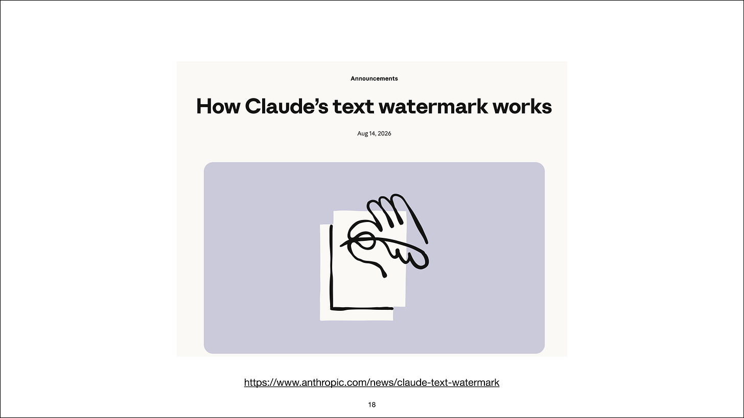
So a few days ago (this is August 14), there was this article, How Claude’s Text Watermark Works, and there was this article here; it’s just like a screen recording, so it can have everything in the slides, but there’s plenty of detail. They updated it actually a couple of times, so originally when I read this, it was a way shorter. Still, it is very, I guess, conceptual; there’s like this overview, and there’s, I mean, there’s not a single figure in there.
And so it’s kind of still hard to understand what they’re trying to do. So they explain a lot about why they’re going to do it, but they don’t explain how. They’re linking to one paper somewhere there, which is very technical also. So I do think it makes sense maybe to take a step back and start at the beginning to kind of understand what they’re trying to implement here with this watermarking technique.
And so the motivation, by the way, of watermarking is for them to identify if someone posts some text that they can say, oh, this text was generated by our Claude Opus 4.8 model, for example, so that they have a way to tell, OK, this text is AI-generated because it carries this watermark. And this watermark is invisible to users, so only they can decode it and find out whether the text has their watermark.
Why can only they do it? We will get to that later in this (hopefully not too long a video), but one thing at a time.
5:38
How LLM Text Generation Works
Slide 4 of 52, time stamp 5:35
So I wanted to start with a brief prelude to explain how text generation works in LLMs, because based on that we can then more easily understand how the watermarking works and that this is actually not a huge, expensive thing on top of it. It’s really just like a minor, I guess, tweak inside the regular text generation process.
Slide 5 of 52, time stamp 6:01
So when we are using something like ChatGPT, for example, let’s say I ask the question, the capital of Germany is, and yeah, ChatGPT or other LLMs, so this is just like an example would, for example, answer “Berlin”. So here, in this case, it’s generating two tokens, like “Berlin” and the period. But for simplicity, let’s assume it’s generating one token. So the next token is the “Berlin” token. How is this token generated internally?
What is happening under the hood when we type something here like the capital of Germany is and receive a token like “Berlin” back? What is actually going on there behind the scenes?
Slide 6 of 52, time stamp 6:41
So in the next couple of slides, I want to briefly talk about what happens under the hood when this next token is generated.
Slide 7 of 52, time stamp 6:50
So assume again that our prompt is the capital of Germany is. And the first step here is to convert this into token IDs. So tokenizing it and converting it into token IDs is one of the main steps at the beginning. This is outside. It’s not inside the LLM; it’s outside of the LLM. So we are simply converting the text into token IDs. It’s just a format that embedding layers can work with.
Slide 8 of 52, time stamp 7:22
And then this passes through the LLM. And the LLM gives us a score distribution for the next token.
Slide 9 of 52, time stamp 7:31
So again, this is just like a brief overview of how LLMs work internally. So I’m not covering the LLM machinery itself. I talked about it many times in my other From Scratch LLMs videos and books. The important part is that when we generate the next token (for example, “Berlin”), we have, at this point, a distribution of scores. So this is the output produced by the LLM.
Here in this case, we’re looking at logit values. So these are just scores from minus infinity to plus infinity, like a range of scores. Here’s an example, ranging from about -8 or -9 to 20. We could convert these into a probability distribution, but technically, it’s not strictly necessary depending on how we sample. But so you can think of the logit values as the raw scores.
And the raw scores go over the entire vocabulary.
Slide 10 of 52, time stamp 8:39
That means every possible word that the LLM could generate. Now here, in the vocabulary index, a certain value (index position 19,846) receives the highest score. So I spread out the distribution. If you would run this prompt through an LLM, you would even see something more extreme: that everything is, like, very, very, very close to zero. And “Berlin” would probably be much, much higher even.
But just to show you a few, you know, like peaks here so it looks a bit more interesting, I kind of zoomed in; in and spread out the distribution a bit. Now here, “Berlin” is the highest score because you can think of it as the most, I guess, probable or plausible next token if I have a very specific prompt like this. So the other ones, I mean, it could be something like Hamburg or Munich that the LLM might guess incorrectly.
But nowadays an LLM should be fairly certain that “Berlin” is the correct answer here. You are also seeing here the vocabulary index. So that’s like over the whole vocabulary. Nowadays, LLMs have like 250,000 possible tokens as output. I’m truncating it here from 19,800 to 19,900 because there’s just so much space here on this slide. If I would have a very realistic vocabulary of 250,000 words, everything would be so narrow that we would barely even be able to tell or see anything on this distribution.
So this is just truncated for educational purposes. The important point is that in regular text generation, we get this score distribution. Now, what we do is look at the highest score.
Slide 11 of 52, time stamp 10:33
I will get into more detail later on how this is selected. So it’s not necessarily precisely the highest one, but for simplicity, assume we are taking the highest score here. And in this case, it’s 19,846.
Slide 12 of 52, time stamp 10:52
And this score is then detokenized, and we get “Berlin” back. So that is the process here on this slide: from an input prompt to conversion into token IDs and tokenization, passing it to the LLM, getting this score distribution, getting the next token, and converting it back into text.
Slide 13 of 52, time stamp 11:12
And then this text is appended to the input. So if we have a question that requires multiple output tokens, we keep going in this loop until the answer is complete. That usually means that the LLM generates an end-of-text token, for example, here. For simplicity, I’m showing you only one iteration where it generates one token. But yeah, as I said, it would kind of continue like that, where we are feeding back the modified input to the LLM for the next round.
Now, how do we actually sample this next token here?
11:39
How Next-Token Sampling Works
Slide 14 of 52, time stamp 11:44
I briefly said, well, we could just technically select the highest one, the one with the highest score. This is called greedy decoding. That’s one way to do it. But most LLMs, like if you use them, they don’t do greedy decoding where they always pick the highest one. Because if you ask it on some other prompt, it might not be what we want to always have the highest score, because then it would memorize the training data.
It would always kind of give the same response and so forth. So we actually often want some variation in the outputs, but not so much that it generates random stuff. So how it works is that, when we sample here from this distribution, we first typically convert it into probability scores.
Slide 15 of 52, time stamp 12:28
So here I just have these scores shown in this plot. I’m just using NumPy for simplicity; whatever tool you use (e.g., PyTorch), the same concepts apply. But let’s assume we have the scores here in NumPy. So what I would do is I would compute the softmax. Technically, I would use a softmax function implemented in Torch or PyTorch, for example, that is numerically stable for both large and small values, including very high positive values, very low positive values, and very high negative values.
Here I’m just writing it out like that. That’s the canonical softmax, just to make it a bit more readable. But the details don’t matter here.
Slide 16 of 52, time stamp 13:20
What matters is that after this conversion, the scores here, I mean, there’s only so much space on the slide, but the scores here, they would add up to one. So it’s essentially like a renormalization. So they would be normalized to sum up to one. That’s all that the probability conversion does: the softmax conversion. So then once we have these probabilities, we can use a random number or, like, a random sampling algorithm.
For example, here in NumPy, we could use the choice function or method. So this is with a specific random seed we are passing to the vocabulary indices. And then, and that’s the important part, we are passing the probabilities as the weights. So, these, essentially, yeah, are like: “How likely is a certain token to be selected?” So, for example, if “Berlin”, after this normalization step, the softmax step, has a 99% probability and the other ones together have a 1% probability, then if we would sample 100 times, 99 of the times, we would get “Berlin”.
In realistic LLMs, for example, that are well trained, “Berlin” might receive a probability of 99.999999 or something like that. So you’re almost certainly always sampling “Berlin” because it’s very confident that the answer is “Berlin” in this particular case. So yeah, that is how we would sample from this distribution. There are modifications like top-k sampling or top-p sampling where, let’s say, just for simplicity in top-k sampling, we would select the top 100 tokens and then apply this random choice only to the top 100, the 100 highest-scoring ones, so that we don’t get nonsense tokens in there.
For this example, it doesn’t really matter. I mean, it’s just like another thing to explain, so I’m skimming over this. So you can maybe assume that this is already the top 100 tokens using top-k or something like that.
Slide 17 of 52, time stamp 15:37
And so, for example, here’s an example. If we sample 10,000 times with a probability of “Berlin” being very high, 99.9, we would sample “Berlin” 9,997 times, sample the word “Hal” twice, and one “Moh”. And these are basically nonsense tokens. It rarely happens that, in this case, the LLM might produce nonsense because, as I mentioned before, I spread out this distribution a bit to make it more interesting.
A real LLM would probably, 10,000 out of 10,000 times, sample “Berlin” because the probability of “Berlin” is so high. But this is for illustration purposes.
16:19
From Sampling to Watermarking
Slide 18 of 52, time stamp 16:21
Now we briefly talked about how LLMs work under the hood, which I think is kind of an interesting concept in itself. But I’ve talked about this many times before, so I don’t want to bore you. I just wanted to set up some context for now, explaining how this watermarking works.
![image](https://substackcdn.com/image/fetch/$s_!WLE_!,w_1456,c_limit,f_auto,q_auto:good,fl_progressive:steep/https%3A%2F%2Fsubstack-post-me
関連記事
今日のまとめ
AIデイリーブリーフで今日の重要ニュースをまとめ読み