現代LLMにおけるアテンション変種のビジュアルガイド

元々、DeepSeek V4 について書く予定でした。しかしまだリリースされていないため、この時間を活用して、長年リストアップしていたプロジェクトに取り組むことにしました。それは過去数年間にわたって取り上げてきたさまざまな LLM アーキテクチャを収集し、整理し、洗練させることです。 そこで、ここ数週間でその取り組みを LLM アーキテクチャギャラリー（執筆時点で 45 エントリー）へとまとめ上げました。これは以前の論文からの資料と、まだ文書化していなかったいくつかの重要なアーキテクチャを組み合わせたものです。各エントリーにはビジュアルモデルカードが付属しており、今後も定期的に更新していく予定です。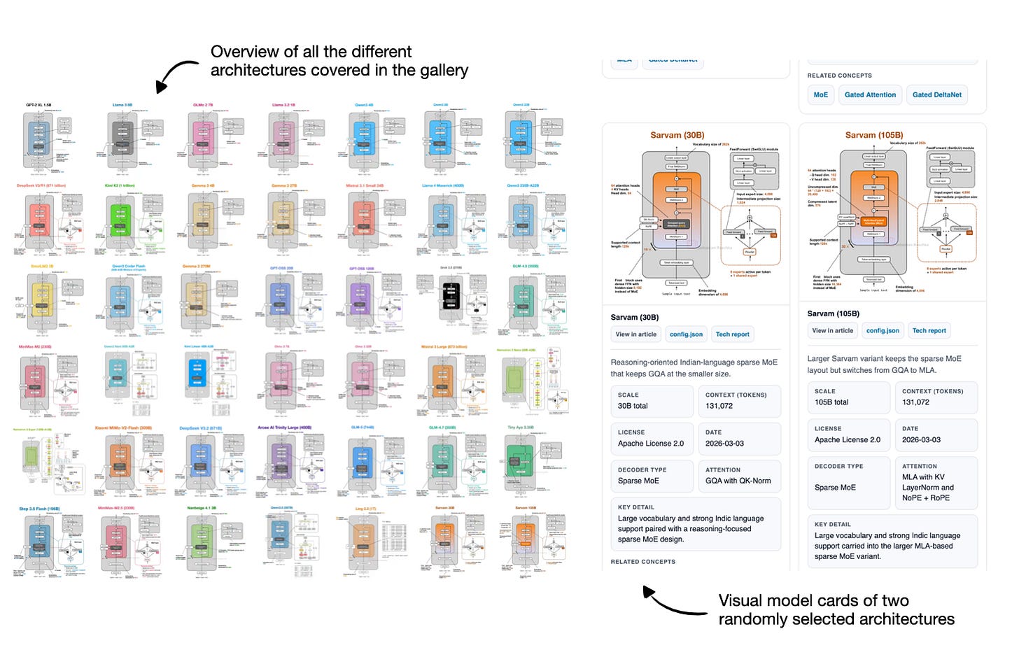 ギャラリーはこちらで見ることができます：https://sebastianraschka.com/llm-architecture-gallery/ ![image](https://substackcdn.com/image/fetch/$s_!wjZ_!,w_1456,c_limit,f_auto,q_auto:good,fl_progressive:steep/https%3A%2F%2Fsubstack-post-media.s3.amazonaws.com%2Fpublic%2Fimages%2F187277b8-e96f-4ef8-8a31-d810076a3057_1494x974.png) 図 1: LLM アーキテクチャギャラリーおよびそのビジュアルモデルカードの概要。 初期バージョンを公開した後、いくつかの読者からポスター版はないかと問い合わせがありました。そこで現在は Redbubble を通じてポスター版も提供しています。私は Medium サイズ（26.9 x 23.4 インチ）を購入して印刷時の様子を確認しましたが、結果は鮮明でクリアでした。ただし、そのサイズでも最も小さなテキスト要素はかなり小さくなっているため、すべての内容を可読にしたい場合は、より小さいバージョンはお勧めしません。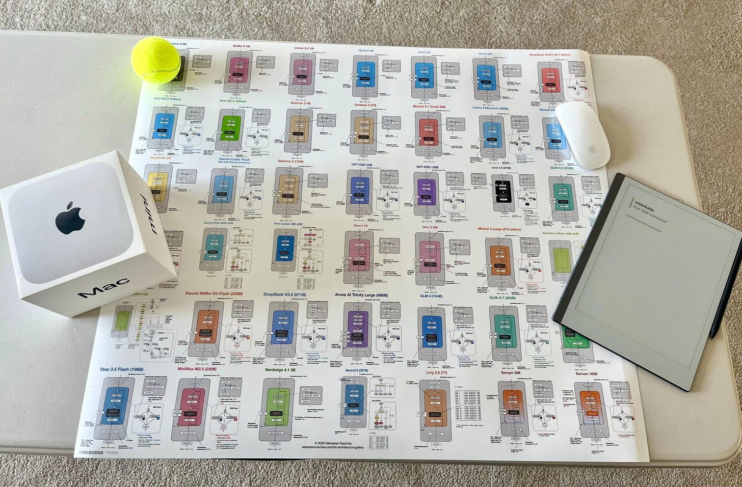 ![image](https://substackcdn.com/image/fetch/$s_!ceew!,w_1456,c_limit,f_auto,q_auto:good,fl_progressive:steep/https%3A%2F%2Fsubstack-post-media.s3.amazonaws.com%2Fpublic%2Fimages%2F03198b65-472c-495e-92c0-62b6af66d720_1999x1313.jpeg) 図 2: アーキテクチャギャラリーのポスター版で、スケールを示すためのいくつかのランダムなオブジェクトが含まれています。 このギャラリーと並行して、私は主要な大規模言語モデル（LLM）の概念に関する短い解説記事も執筆中です。 そこで今回は、近年注目されるオープンウェイトアーキテクチャで開発・採用された最新の注意機構（アテンション）の変種をすべて振り返ることで、興味深い内容になるだろうと考えました。 私の目標は、このコレクションがリファレンスとしても、軽量な学習リソースとしても有用となるようにすることです。皆様にとって有益かつ教育的なものになれば幸いです！ 1. マルチヘッドアテンション（MHA） セルフアテンションでは、各トークンがシーケンス内の他の可視トークンを参照し、それらに重みを割り当て、その重みを用いて入力に対する新しい文脈依存表現を構築します。 マルチヘッドアテンション（Multi-Head Attention: MHA）は、この考え方を標準的なトランスフォーマー版として実装したものです。複数のセルフアテンションヘッドを並列で実行し、それぞれが異なる学習された射影を用いて処理を行い、その出力を組み合わせてより豊かな表現へと統合します。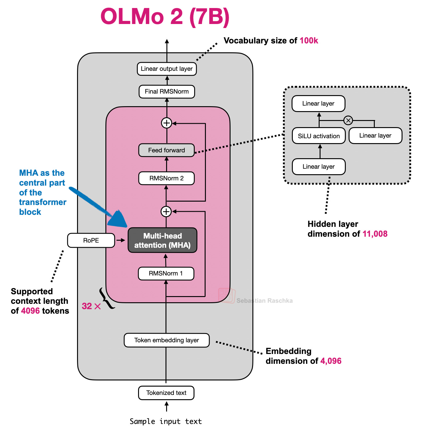 ![image](https://substackcdn.com/image/fetch/$s_!GrJT!,w_1456,c_limit,f_auto,q_auto:good,fl_progressive:steep/https%3A%2F%2Fsubstack-post-media.s3.amazonaws.com%2Fpublic%2Fimages%2Fa3ed41e9-86ee-4c1c-80a5-c9c2ed59dd9c_1366x1410.png) 図 3: MHA を採用するアーキテクチャの例としての Olmo 2。 以下のセクションでは、まず MHA（Multi-Head Attention）を説明するために自己注意機構（self-attention）の概要を素早く巡ります。これは、グループ化クエリアテンション（grouped-query attention）、スライディングウィンドウアテンション（sliding window attention）などの関連する注意概念のための舞台設定を行うための簡易な概説として意図されています。より長く詳細な自己注意機構の解説に興味がある場合は、私の「LLM における自己注意機構、マルチヘッドアテンション、因果的アテンション、クロスアテンションの理解と実装」という長編記事をご覧になることをお勧めします。 例示アーキテクチャ GPT-2, OLMo 2 7B, および OLMo 3 7B 1.2 歴史的な豆知識とアテンションが考案された理由 アテンションはトランスフォーマーや MHA よりも以前に存在します。その直近の背景には、翻訳のためのエンコーダー・デコーダー RNN（Recurrent Neural Network）があります。 これらの古いシステムでは、エンコーダー RNN がソース文をトークンごとに読み込み、それを隠れ状態のシーケンス、あるいは最も単純なバージョンでは最終的な一つの状態に圧縮します。その後、デコーダー RNN はその限定的な要約からターゲット文を生成する必要がありました。これは短く単純なケースでは機能しましたが、次の出力単語に関連する情報が入力文の別の場所にある場合、明白なボトルネックが生じました。 つまり、問題は隠れ状態が無限の情報やコンテキストを保持できない点にあり、時には完全な入力シーケンスを参照し直すことが有用になることがあるのです。 以下の翻訳例は、このアイデアの限界の一つを示しています。例えば、文は多くの局所的に妥当な語彙選択を保持していても、モデルが問題を単語ごとの対応として過度に扱う場合、翻訳として失敗することがあります。（上段のパネルでは、文を単語ごとに翻訳する誇張された例を示していますが、明らかに結果の文の文法は誤っています。）実際には、正しい次の単語は、文レベルの構造と、そのステップでどの先行ソース単語が重要であるかに依存します。もちろん、これは RNN でも適切に翻訳可能ですが、前述したように隠れ状態が保持できる情報量に限界があるため、より長いシーケンスや知識検索タスクでは困難を伴います。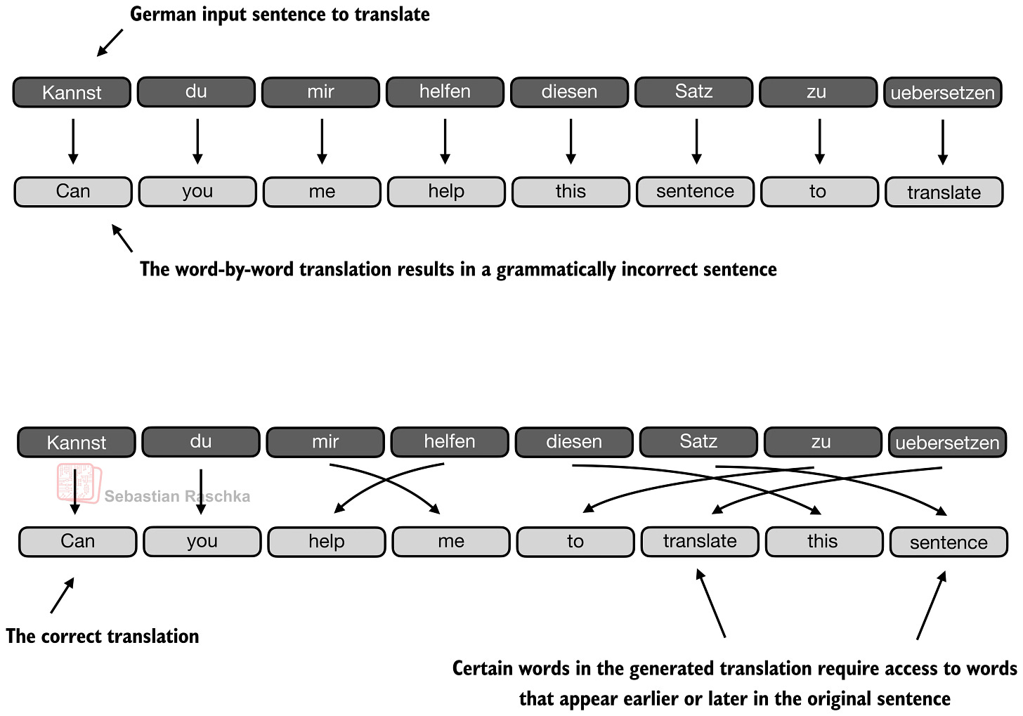 ![image](https://substackcdn.com/image/fetch/$s_!jdH6!,w_1456,c_limit,f_auto,q_auto:good,fl_progressive:steep/https%3A%2F%2Fsubstack-post-media.s3.amazonaws.com%2Fpublic%2Fimages%2F95e6491c-6457-4af0-83f3-b73310bad668_3566x2495.webp) 図 4: 個々の語彙選択の多くが妥当に見える場合でも、文レベルの構造が依然として重要であるため、翻訳は失敗する可能性があります（元のソース：LLMs-from-scratch）。 次の図は、この変化をより直接的に示しています。デコーダーが出力トークンを生成する際、1 つの圧縮された記憶経路に限定されるべきではありません。より関連性の高い入力トークンに直接遡ってアクセスできる必要があります。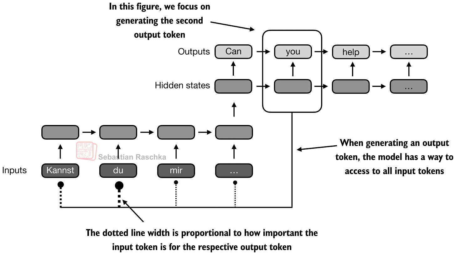 ![image](https://substackcdn.com/image/fetch/$s_!T2XV!,w_1456,c_limit,f_auto,q_auto:good,fl_progressive:steep/https%3A%2F%2Fsubstack-post-media.s3.amazonaws.com%2Fpublic%2Fimages%2Feaafc89d-0765-4e90-8f2b-881032cb2d5b_3415x1914.webp) 図 5: アテンション（attention）は、現在の出力位置が単一の圧縮された状態に頼るのではなく、入力シーケンス全体を再訪できるようにすることで、RNN のボトルネックを打破します（元出典：LLMs-from-scratch）。 トランスフォーマー（Transformers）は、前述のアテンション修正型 RNN からその核となるアイデアを引き継ぎつつも、再帰性（recurrence）を取り除いています。古典的な「Attention Is All You Need」論文において、アテンション自体が主要なシーケンス処理メカニズムとなります（RNN エンコーダー・デコーダーの一部であるだけでなく）。 トランスフォーマーでは、このメカニズムは自己アテンション（self-attention）と呼ばれ、シーケンス内の各トークンが他のすべてのトークンに対して重みを計算し、それらのトークンからの情報を混合して新しい表現を生成します。マルチヘッド・アテンション（multi-head attention）とは、同じメカニズムを並列に複数回実行するものです。 1.3 マスク付きアテンション行列 T トークンのシーケンスに対して、アテンションでは各トークンごとに重みの行が必要となるため、全体として T x T の行列が得られます。 各行は単純な問いに応えるものです。このトークンを更新する際、各可視トークンはどの程度重要なのか？デコーダー専用 LLM では、未来の位置はマスク（mask）されるため、下の図では行列の右上部分が灰色で表示されています。 自己アテンションは、因果マスクの下でこれらのトークン間重みパターンを学習し、それらを用いて文脈を考慮したトークン表現を構築することの本質です。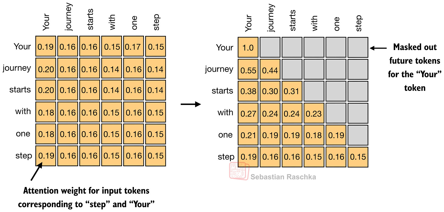 ![image](https://substackcdn.com/image/fetch/$s_!8wZw!,w_1456,c_limit,f_auto,q_auto:good,fl_progressive:steep/https%3A%2F%2Fsubstack-post-media.s3.amazonaws.com%2Fpublic%2Fimages%2Fd6e9affd-687b-4170-b1d5-f8e3d2834d2b_3449x1646.webp) 図 6: 具体的なマスク付きアテンション行列の例。各行は一つのトークンに属し、各エントリはアテンション重みであり、因果マスクによって未来のトークンに関するエントリが除去されています（元出典：Understanding and Coding Self-Attention）。 1.4 自己アテンションの内部構造 次の図は、トランスフォーマーが入力埋め込み X からアテンション行列 (A) を計算し、それが変換された入力 (Z) の生成にどのように用いられるかを示しています。 ここで Q、K、V はそれぞれクエリ（queries）、キー（keys）、値（values）を意味します。トークンのクエリは、そのトークンが何を探しているかを表し、キーは各トークンがマッチングのために何を利用可能にしているかを表し、値はアテンション重みが計算された後に出力に混合される情報を表します。 手順は以下の通りです： Wq、Wk、および Wv は、入力埋め込みを Q、K、V へ投影する重み行列です。 QK^T は、トークン間の生の関連度スコアを生成します。 softmax は、これらのスコアを前節で議論した正規化されたアテンション行列 A に変換します。 A が V に適用され、出力行列 Z が生成されます。 注意してください。アテンション行列は、手書きの別個のオブジェクトではありません。これは Q（クエリ）、K（キー）、および softmax から生じるものです。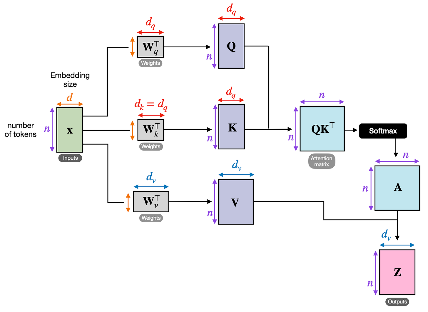 ![image](https://substackcdn.com/image/fetch/$s_!ZbSh!,w_1456,c_limit,f_auto,q_auto:good,fl_progressive:steep/https%3A%2F%2Fsubstack-post-media.s3.amazonaws.com%2Fpublic%2Fimages%2F635f204a-bd68-4162-ac88-ca5da9ba6be8_1498x1092.png) 図 7: 入力埋め込み X から正規化されたアテンション行列 A、および出力表現 Z に至る完全な単一ヘッドのパイプライン（元出典：Understanding and Coding Self-Attention）。 次の図は、前の図と同じ概念を示していますが、アテンション行列の計算が「スケーリングドットプロダクトアテンション」ボックスの中に隠されており、すべての入力トークンに対してではなく、1 つの入力トークンのみに対して計算を実行します。これは、次のセクションでマルチヘッドアテンションに拡張する前に、単一ヘッドによる自己アテンションのコンパクトな形式を示すためです。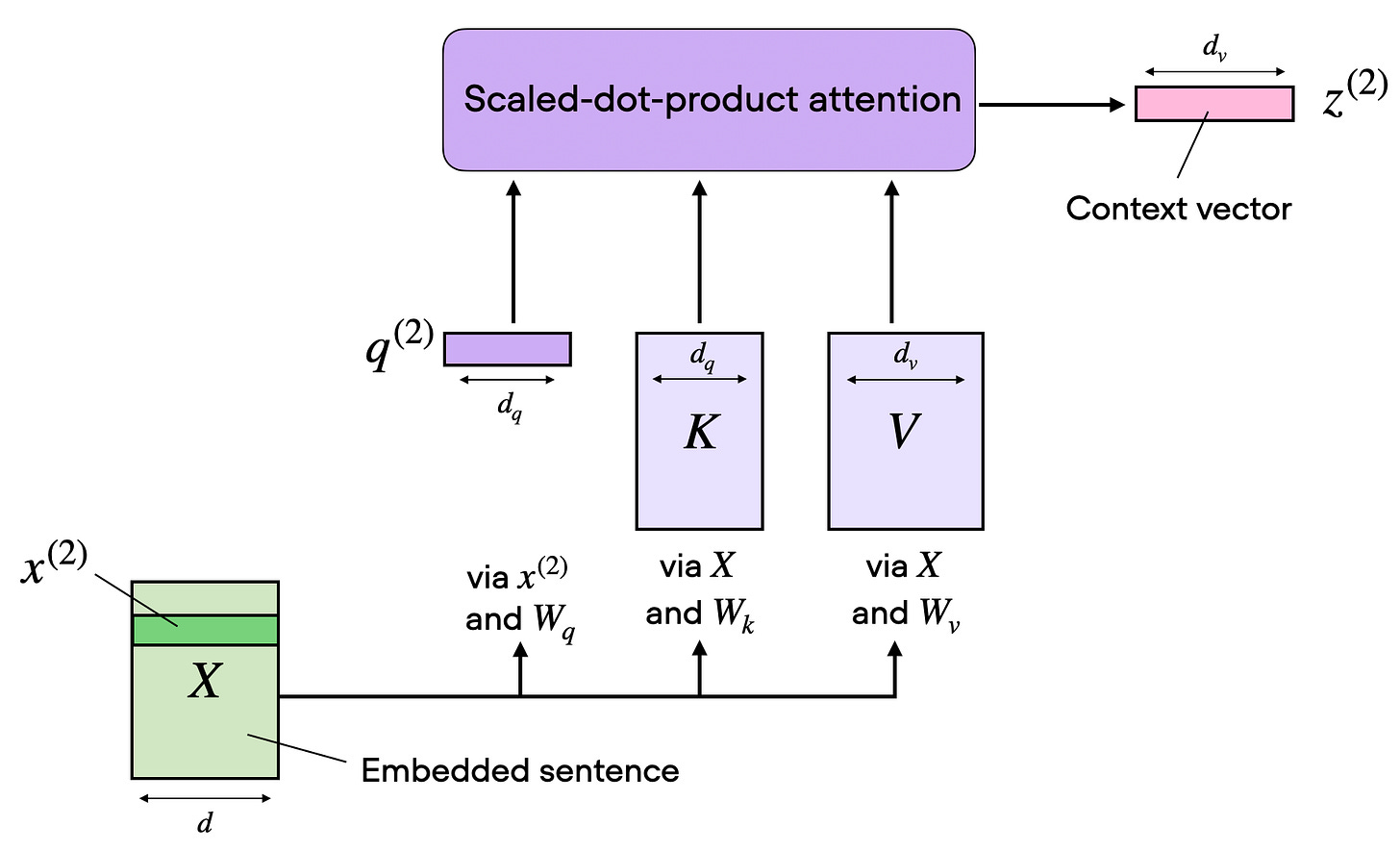 ![image](https://substackcdn.com/image/fetch/$s_!VJyp!,w_1456,c_limit,f_auto,q_auto:good,fl_progressive:steep/https%3A%2F%2Fsubstack-post-media.s3.amazonaws.com%2Fpublic%2Fimages%2F7dfb70d9-5eb6-44df-a880-3a37dfe72d7f_1836x1116.png) 図 8: 1 つのアテンションヘッドはすでに完全なメカニズムです。1 つのセットの学習済み射影（投影）が、1 つのアテンション行列と 1 つの文脈認識型出力ストリームを生成します（元出典：Understanding and Coding Self-Attention）。 1.5 単一ヘッドからマルチヘッドアテンションへ Wq/Wk/Wv の行列セット 1 つが 1 つのアテンションヘッドを与え、つまり 1 つのアテンション行列と 1 つの出力行列 Z を意味します。（この概念は前のセクションで説明されています。） マルチヘッドアテンションは、単に異なる学習された射影行列を用いてこれらのヘッドを並列に複数実行するものです。 これは有用です。なぜなら、異なるヘッドが異なるトークン間の関係性に特化できるからです。あるヘッドは短い局所的な依存関係に焦点を当て、別のヘッドはより広範な意味的なリンクに、さらに別のヘッドは位置情報や構文構造に焦点を当てる可能性があります。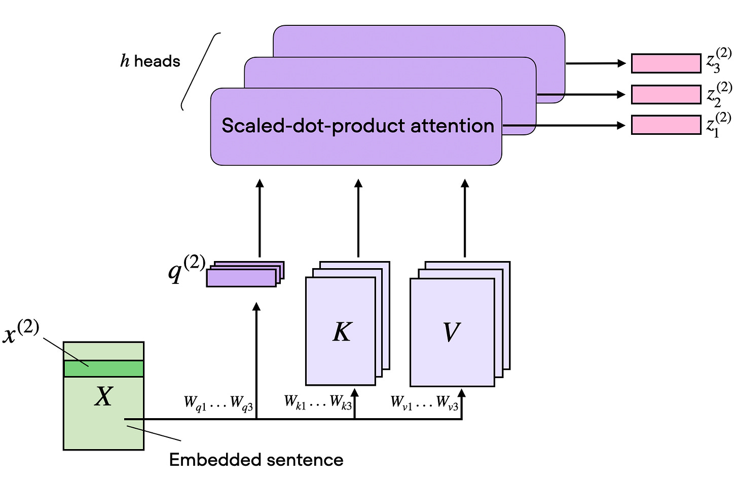 ![image](https://substackcdn.com/image/fetch/$s_!MSOX!,w_1456,c_limit,f_auto,q_auto:good,fl_progressive:steep/https%3A%2F%2Fsubstack-post-media.s3.amazonaws.com%2Fpublic%2Fimages%2F5f47ffd2-bb3a-4936-9720-a88b8d867337_1766x1154.png) 図 9: マルチヘッドアテンションは、基本的なアテンションのレシピを維持しつつ、これを並列で複数のヘッドに繰り返すことで、モデルが一度に複数のトークン間パターンを学習できるようにします（元出典：Understanding and Coding Self-Attention）。 2. グループ化クエリアテンション (GQA) グループ化クエリアテンションは、標準的なマルチヘッドアテンション (MHA) から派生したアテンションのバリアントです。これは 2023 年に Joshua Ainslie らによって発表された論文「GQA: Training Generalized Multi-Query Transformer Models from Multi-Head Checkpoints」で導入されました。 すべてのクエリヘッドに個別のキーと値を与えるのではなく、複数のクエリヘッドが同じキー・値射影を共有することを可能にし、これにより KV キャッシング (Key-Value Caching) が大幅に低コスト化されます（主にメモリ削減として）、全体のデコーダーのレシピにはほとんど変更を加えずに済みます。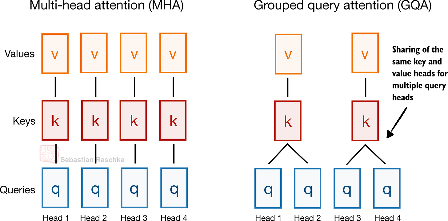 ![image](https://substackcdn.com/image/fetch/$s_!h6wM!,w_1456,c_limit,f_auto,q_auto:good,fl_progressive:steep/https%3A%2F%2Fsubstack-post-media.s3.amazonaws.com%2Fpublic%2Fimages%2F6f39923c-8357-487d-9e69-40ee18a902e8_2523x1248.png) 図 10: GQA は MHA と同じ全体的なアテンションパターンを維持しつつ、複数のクエリヘッド間でキー・バリューヘッドを共有することで、その数を削減します（出典：The Big LLM Architecture Comparison）。 EXAMPLE ARCHITECTURES Dense: Llama 3 8B, Qwen3 4B, Gemma 3 27B, Mistral Small 3.1 24B, SmolLM3 3B, Tiny Aya 3.35B。 Sparse (Mixture-of-Experts): Llama 4 Maverick, Qwen3 235B-A22B, Step 3.5 Flash 196B, Sarvam 30B。 2.1 なぜ GQA が普及したのか 私のアーキテクチャ比較記事では、GQA を古典的なマルチヘッドアテンション（MHA）の新しい標準的な代替案として位置づけました。その理由は、標準的な MHA では各ヘッドが独自のキーとバリューを持つため、モデル化の観点からはより最適ですが、推論時に KV キャッシュにすべての状態を保持しなければならない場合、コストが高くなるからです。 GQA では、より多くのクエリヘッドを維持しつつ、キー・バリューヘッドの数を減らし、複数のクエリでそれらを共有します。これにより、パラメータ数と KV キャッシュのトラフィックを削減できますが、後ほど議論するマルチヘッド潜在アテンション（MLA）のような劇的な実装変更は必要ありません。 実際には、MHA よりも安価でありながら、MLA のような新しい圧縮重視の代替案よりも実装が簡単であるという点から、この手法はラボにとって非常に人気のある選択肢となり続けています。 2.2 GQA によるメモリ節約 GQA は KV ストレージにおいて大きな節約をもたらします。なぜなら、各レイヤーで保持するキー・バリューヘッドの数が少なければ少ないほど、トークンあたりに必要なキャッシュ状態量が減るからです。これが、シーケンス長が成長するにつれて GQA の有用性が高まる理由です。 GQA はスペクトラム（連続体）として捉えることもできます。もしすべてのキー・バリューグループを 1 つの共有グループまで削減すれば、私たちは実質的にマルチクエリアテンションの領域に到達することになります。これはさらに安価ですが、モデル化の品質に対してより顕著な悪影響を与える可能性があります。最適なバランス点は通常、マルチクエリアテンション（1 つの共有グループ）と MHA（キー・バリューグループ数がクエリ数に等しい状態）の間にあるものであり、ここではキャッシュ節約効果が大きい一方で、MHA に対するモデル化性能の低下は控えめに抑えられています。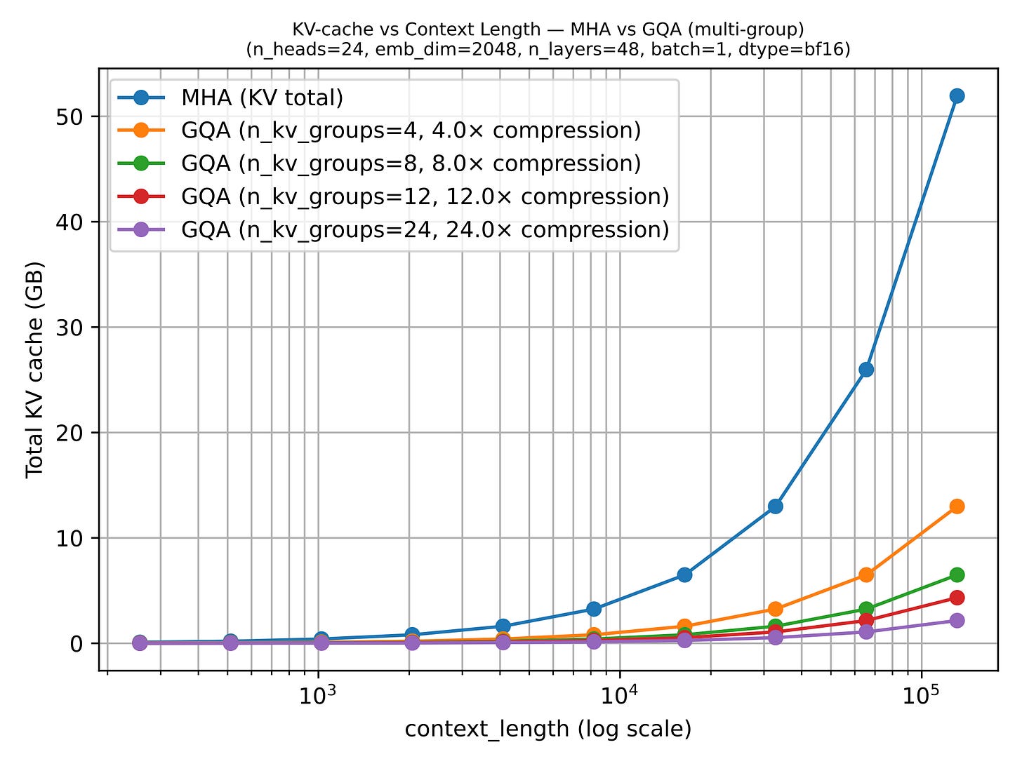 ![image](https://substackcdn.com/image/fetch/$s_!87ib!,w_1456,c_limit,f_auto,q_auto:good,fl_progressive:steep/https%3A%2F%2Fsubstack-post-media.s3.amazonaws.com%2Fpublic%2Fimages%2F95380983-7afc-4456-9d5b-733216c16a91_1920x1440.png) 図 11: 数値が低いほど優れています。コンテキストウィンドウが大きくなるにつれて、KV キャッシュの節約効果がより顕著になります。（出典：LLMs-from-scratch GQA マテリアル） 2.3 なぜ 2026 年においても GQA は重要なのか より高度なバリアントである MLA は、同じ KV エフィシエンシーレベルにおいてより優れたモデリング性能を提供できるため（例えば DeepSeek-V2 論文の消融実験で議論されている通り）、人気を集めつつありますが、その反面、実装がより複雑になり、アテンションスタックもより複雑なものになります。 GQA は、堅牢であり、実装が容易で、トレーニングも容易である（私の経験則では、必要なハイパーパラメータの調整が少ないため）という点から依然として魅力的です。 そのため、一部の最新リリースでもあえてクラシックなアプローチを維持しています。例えば、私の「Spring Architectures」記事で言及した MiniMax M2.5 や Nanbeige 4.1 は、他の効率化トリックを追加せず、グループドクエリアテンション（Grouped-Query Attention）のみを使用する非常にクラシックなモデルです。Sarvam も特に有用な比較対象となります：30B モデルはクラシックな GQA を維持している一方、105B バージョンでは MLA に切り替えています。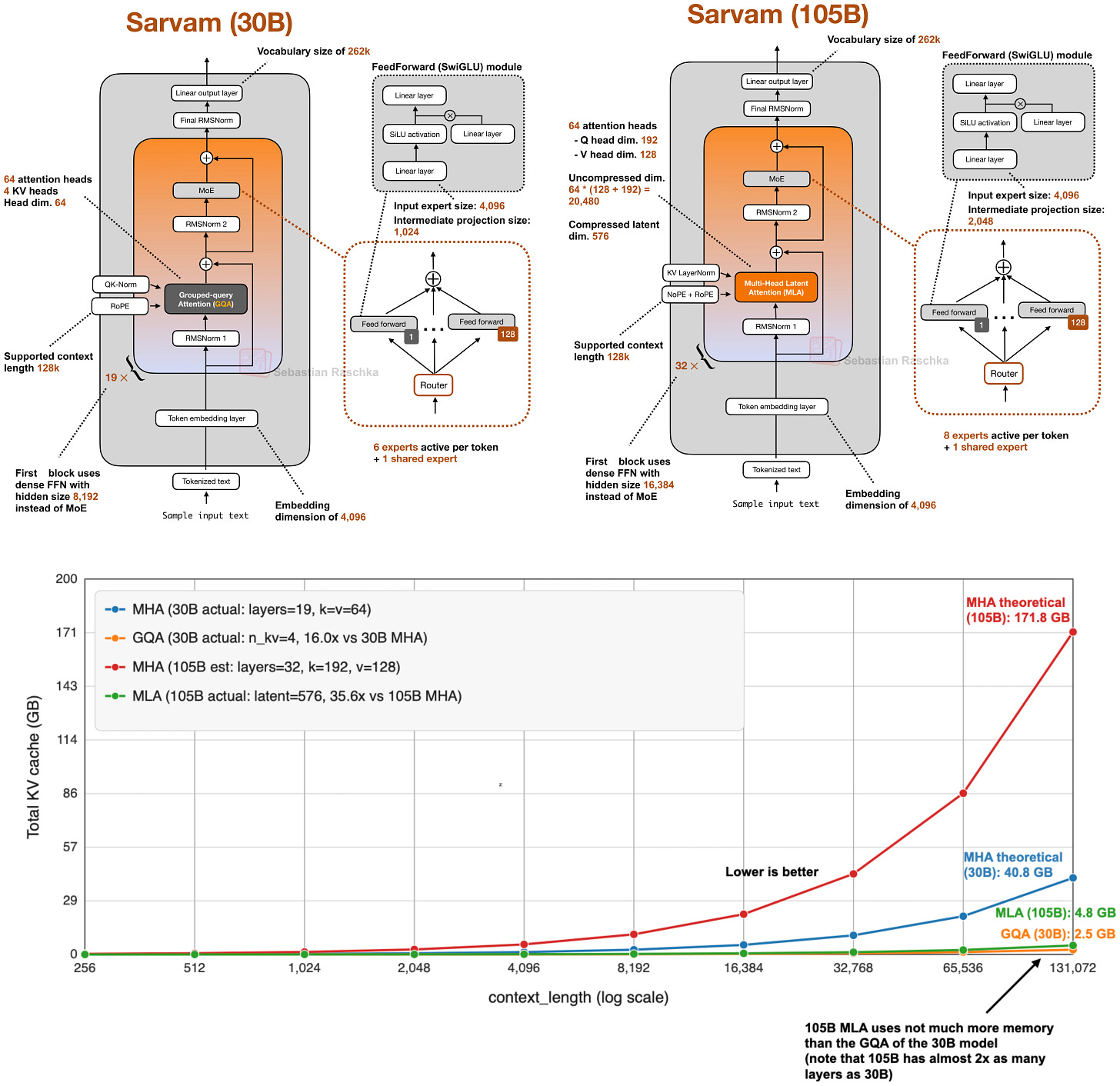 ![image](https://substackcdn.com/image/fetch/$s_!BMEL!,w_1456,c_limit,f_auto,q_auto:good,fl_progressive:steep/https%3A%2F%2Fsubstack-post-media.s3.amazonaws.com%2Fpublic%2Fimages%2F2d04f89a-aad5-4af7-8b46-4623d1d53ae9_5860x5682.webp) 図 12: 105B Sarvam（MLA 使用）と 30B Sarvam（GQA 使用）、および通常の MHA（Multi-Head Attention）を使用した場合の総 KV キャッシュサイズ。 3. マルチヘッド潜在アテンション (MLA) Multi-head Latent Attention (MLA) の背後にある動機は、Grouped-Query Attention (GQA) と同様です。両者とも KV-cache のメモリ要件を削減するための解決策です。GQA と MLA の違いは、MLA がヘッドを共有して保存する K/V の数を減らすのではなく、保存される内容を圧縮することでキャッシュを縮小する点にあります。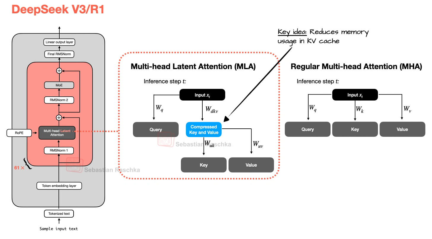 ![image](https://substackcdn.com/image/fetch/$s_!FcJB!,w_1456,c_limit,f_auto,q_auto:good,fl_progressive:steep/https%3A%2F%2Fsubstack-post-media.s3.amazonaws.com%2Fpublic%2Fimages%2Fe29cb535-8854-4412-af8d-9bca8d8d05f2_1550x858.webp) 図 13: GQA と異なり、MLA はヘッドをグループ化することで KV コストを削減するわけではありません。代わりに、圧縮された潜在表現（latent representation）をキャッシュすることでコストを削減します。簡略化のため省略されていますが、これはクエリにも適用されます（元出典：The Big LLM Architecture Comparison）。 MLA はもともと DeepSeek-V2 の論文で提案されましたが、DeepSeek 時代の象徴的なアイデアとなりました（特に DeepSeek-V3 と R1 以降）。GQA に比べて実装は複雑であり、サービス提供もより困難ですが、モデルサイズやコンテキスト長が十分に大きくなりキャッシュのトラフィックが支配的になる現代においては、むしろ魅力的な選択肢となることが多くなっています。同じメモリ削減率であっても、より優れたモデリング性能を維持できるからです（これについては後述します）。 EXAMPLE ARCHITECTURES DeepSeek V3, Kimi K2, GLM-5, Ling 2.5, Mistral Large 3, および Sarvam 105B 3.1 共有ではなく圧縮 MHA や GQA がフル解像度のキーおよびバリューテンソルをキャッシュするのとは異なり、MLA は潜在表現を保存し、必要に応じて使用可能な状態を再構築します。本質的には、これはアテンション内部に埋め込まれたキャッシュ圧縮戦略であり、前述の図で示されています。 以下の図は、通常の MHA と比較した削減効果を表しています。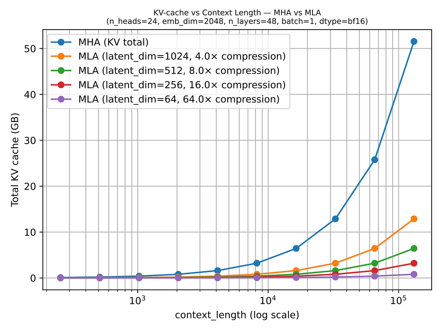 ![image](https://substackcdn.com/image/fetch/$s_!56rA!,w_1456,c_limit,f_auto,q_auto:good,fl_progressive:steep/https%3A%2F%2Fsubstack-post-media.s3.amazonaws.com%2Fpublic%2Fimages%2F186dfe98-db29-4b12-97ab-39d5b21ab460_1920x1440.png) 図 14: コンテキスト長が成長すると、フル K/V テンソルではなく潜在表現をキャッシュすることによる削減効果が非常に明確になります（元出典：LLMs-from-scratch の MLA セクション）。 3.2 MLA アブレーションスタディーズ DeepSeek-V2 の論文では、いくつかのアブレーション実験が示されており、モデル性能の観点からは GQA が MHA よりも劣っているように見える一方で、MLA ははるかに良好に機能し、注意深くチューニングすれば MHA をさえ上回る可能性があるとされています。これは「（メモリも）節約できる」という理由よりも、はるかに強力な根拠となります。 つまり、DeepSeek にとって MLA が好ましいアテンションメカニズムである理由は、単に効率的だからだけでなく、大規模スケールにおいて品質を維持したままの効率化策として機能するように見えるからです。（ただし、同僚からは、MLA は特定のサイズでのみうまく機能すると聞いています。より小さなモデル、例えば 100B より小さい場合では、GQA の方がむしろよく機能するか、少なくともチューニングして正しく動作させるのが容易であるようです。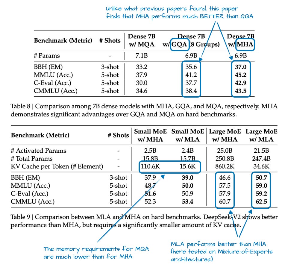） ![image](https://substackcdn.com/image/fetch/$s_!1yW7!,w_1456,c_limit,f_auto,q_auto:good,fl_progressive:steep/https%3A%2F%2Fsubstack-post-media.s3.amazonaws.com%2Fpublic%2Fimages%2Ff564ec9f-5fcb-49c3-b728-b4c8a769bb6c_952x902.png) 図 15: ここでは GQA が MHA を下回っており、MLA は依然として競争力があり、わずかに上回ることもあります。基礎となる論文：DeepSeek-V2。 以下は、30B の Sarvam における GQA と、105B の Sarvam における MLA の比較を再掲したものです。 ![image](https://substackcdn.com/image/fetch/$s_!cbqs!,w_1456,c_limit,f_auto,q_auto:good,fl_progressive:steep/https%3A%2F%2Fsubstack-post-media.s3.amazonaws.com%2Fpublic%2Fimages%2Fa425874e-baae-45bb-a199-46648c5db725_5860x5682.webp) 図 16: GQA と MLA は、異なる方向から同じボトルネックを解決しています。トレードオフは、簡素さ versus より大規模なモデルにおける優れたモデリング性能です。 3.3 DeepSeek 後の MLA の普及 DeepSeek V3/R1 や V3.1 などにより、V2 で導入された設計が標準化されると、MLA は第二波のアーキテクチャにおいて現れ始めました。Kimi K2 は DeepSeek のレシピを継承してスケールアップしました。GLM-5 は、DeepSeek Sparse Attention（DeepSeek V3.2 から）とともに MLA を採用しました。Ling 2.5 は、MLA と線形アテンションのハイブリッドを組み合わせています。Sarvam は 2 つのモデルをリリースしており、30B モデルは従来の GQA に留まり、105B モデルは MLA に切り替えました。 最後のペアは特に有用です。なぜなら、技術的な複雑さに関する議論を脇に置くことができるからです。つまり、Sarvam チームは両方のバリアントを実装し、意図的に一方には GQA を、他方には MLA を採用することを選択しました。したがって、ある意味で、MLA は理論的な代替案というよりも、ファミリーがスケールアップする際に具体的なアーキテクチャのアップグレードパスのように感じられます。 4. スライディングウィンドウアテンション (SWA) スライディングウィンドウアテンションは、各位置が参照できる過去のトークンの数を制限することで、長文コンテキスト推論におけるメモリと計算コストを削減します。すべてのプレフィックスに注意を向けるのではなく、各

現代LLMにおけるアテンション変種のビジュアルガイド

背景や根拠まで確認しますか？

関連記事

調べる

選ぶ

サイト