GridSFM:電力系統向けに新登場した軽量基盤モデル
Microsoft Research は、送電網の AC 最適電力流れ問題をミリ秒単位で解決し、年間最大 200 億ドルのコスト削減と再生可能エネルギーの有効活用を可能にする軽量基盤モデル「GridSFM」を発表した。
キーポイント
AC-OPF の高速化実現
従来の計算に数時間かかる複雑な非凸最適化問題(AC-OPF)を、ミリ秒単位で近似解決可能にし、リアルタイム運用のボトルネックを解消します。
経済的・環境的影響
送電網の混雑損失を年間最大 200 億ドル削減し、3.4TWh に及ぶ再生可能エネルギーの廃棄(カータルメント)を大幅に減らす可能性を秘めています。
システム状態の可視化
単なる発電量推定だけでなく、混雑、安定性、系統全体の健康状態を含む完全な AC システム状態を生成し、運用者の意思決定を直接支援します。
コミュニティ基盤の提供
既存のデータやモデルから再構築する必要なく、高度な電力網シミュレータや計画ツールの開発を可能にするオープンな基盤として機能します。
高速なAC-OPF近似とリアルタイム評価
GridSFMは500〜80,000バスの電力系統に対してミリ秒単位で交流最適潮流(AC-OPF)を近似し、計算ボトルネックを解消することでリアルタイムでの多数シナリオ評価を可能にします。
単一モデルによる汎化と学習アプローチ
150以上の基本トポロジーと約50万のシナリオで訓練された単一のブロック構造ニューラル演算子であり、物理法則や制約違反を罰する損失関数を用いて特定の系統への過学習を防ぎ汎化能力を高めています。
高い精度と既存手法との比較優位性
テストシナリオでソルバー基準値に対し中央値2.23%のコストギャップを達成し、従来の数値ソルバーのウォームスタートやDC-OPFと比較して1.5倍以上の性能向上を示しています。
影響分析・編集コメントを表示
影響分析
この発表は、電力インフラの運用効率化における AI の実用化における画期的な転換点となります。従来の数時間かかる計算をミリ秒に短縮することで、再生可能エネルギーの大量導入や気候変動への対応といった喫緊の課題に対し、リアルタイムかつ経済的に最適な制御を可能にし、電力システムの信頼性と持続可能性を根本から支える基盤技術として確立されます。
編集コメント
電力システムという極めて重要かつ複雑なインフラ領域において、AI が物理法則を尊重しつつ計算速度を劇的に向上させた事例は貴重です。これは単なる技術デモではなく、即座に社会実装可能なインパクトを持つ成果と言えます。

Microsoft は、ミリ秒単位で交流最適潮流(AC optimal power flow)を予測できる軽量なファウンデーションモデルを発表し、グリッド分析における効率向上とコスト削減の可能性を開きました。
At a glance
Microsoft は GridSFM を導入しました。これは、交流最適潮流をミリ秒単位で近似する小型のファウンデーションモデルであり、年間最大 200 億ドルに達する混雑損失や 3.4 テラワット時の再生可能エネルギーの抑制(curtailment)に直接影響を与える意思決定の可能性を開くものです。
発電機の稼働計画とコストの見積もりを超えて、GridSFM は完全な交流システム状態を生成し、運用担当者が混雑、安定性、および全体のシステムの健全性を直接的に把握できるようにします。
これは、データやモデルを一から作り直すことなく、コミュニティが高度な電力グリッドシミュレータや計画ツールを構築するための基盤を提供するものです。
Microsoft は GridSFM を導入しました。これは送電網における交流最適潮流(AC-OPF)問題を解決するための小型ファウンデーションモデルです。これは、GridSFM の動力源となる米国ベースのオープンな送電トポロジデータセットを以前に発表した後の続報となります。
電力グリッドは、需要の急増、再生可能エネルギー源の統合、交通の電気化、そして極端な気象事象への対応から、ますます大きな負荷に直面しています。これらのすべての課題において、核心的な問いは同じです。各新しい条件下でグリッドが機能し続けるための最適な運転点とは何でしょうか?
これに答えるには、交流最適電力潮流(AC-OPF)を解く必要があります。これは複雑な非凸最適化問題であり、需要を満たしつつ電力潮流の物理法則、電圧制限、熱的制約、安定性要件を遵守しながら、最も安価な発電機出力配分(各発電機の生産量)を計算するものです。この問題は、信頼性、リアルタイム配分、市場清算、事故分析などの中核的な電力システム運用の基盤となっています。これらの意思決定は、年間最大 200 億ドル規模の混雑コストや数テラワット時の再生可能エネルギーの抑制(混雑による再生可能エネルギーの損失)という結果を直接支配しており、経済効率性とグリッド信頼性の両方が、これらの運転点をいかに正確に見つけるかに極めて敏感であることを意味しています。しかし、AC-OPF は計算コストが高く、大規模な電力ユーティリティ用グリッドでは解決に数時間かかることもあり、慎重に選択された少数のシナリオを解くか、重要な物理法則を無視する近似手法に頼るかのトレードオフを迫られます。後者の場合、電力潮流や拘束条件の見積もりが誤り、ストレス条件下で最適でない配分や信頼性の低下を招く可能性があります。
注目:AI 搭載エクスペリエンス

Microsoft Research Copilot エクスペリエンス
AI を活用したエクスペリエンスを通じて、Microsoft の研究についてさらに詳しくご紹介します
今すぐ開始
新しいタブで開く
この制限に対処するため、500 バスから 80,000 バスまでの広範囲の電力系統において数ミリ秒で交流最適潮流(AC-OPF)を近似する単一のニューラルネットワークである GridSFM を導入します。標準的な AC-OPF の入力(系統トポロジ、発電機および負荷仕様、送電線制約)を受け取り、運転点と実行可能性の判定(システムがすべての物理的・運用上の制約を満たすかどうか)を出力します。計算リソースのボトルネックを排除することで、GridSFM はリアルタイムで桁違いに多くのシナリオを評価可能にし、より情報に基づいた意思決定を可能にする一方、系統運用を反応的な対応から予防的な最適化へと転換させます。
今回の初期リリースでは 2 つのティアを提供します:
研究規模の系統(最大 4,000 バス)向けの GridSFM-Open。
生産規模のシステム(最大 80,000 バス)向けの GridSFM-Premier。
このモデルは、ブロック構造を持つ離散型ニューラル演算子(図 1)として構築されており、各電力系統を有向グラフとして表現します。ここで、バス(系統内の接続点)と発電機が頂点となり、送電線や交流線がエッジとなります。学習には、ソルバーによる監督学習と物理ベースの制約の両方が用いられます。監督学習では、AC-OPF ソルバー(PowerModels.jl の IPOPT を使用)を用いて参照解を生成します。一方、物理ベースの制約は、キルヒホッフの電圧・電流則といった基本的な物理法則や、熱的制限などの運用上の制約に対する違反に対してペナルティを与えるものです。これにより、モデルは実行可能領域と不可能領域の両方から学習することが可能になります。多くの学習ベースの AC-OPF 代理モデルは、限られた分布において各系統ごとに 1 つずつモデルを訓練します。一方、GridSFM はこれとは対照的なアプローチを採用しています:今回のリリースでは、単一のモデルが 150 以上の基本系統トポロジ(ネットワーク構造)と、変動する負荷プロファイル、多要素停電、線路定格の降格、電圧制約の厳格化、異なる発電機コスト係数などを含む約 50 万シナリオにわたって訓練されています。これにより、モデルは暗記ではなく一般化を迫られることになります。GridSFM-Open の 54 系統混合テストシナリオ全体において、当モデルはソルバーの正解ラベルと比較して中央値で 2.23% のコストギャップ(平均 3.41%)を達成しました。従来の数値ソルバーに対するウォームスタートシード(GridSFM-seeded-warm)は、同じテストシナリオ全体での幾何平均においてコールドソルブよりも 1.66 倍優れており、業界標準の DC-OPF ウォームスタートよりも 1.59 倍優れています。詳細な系統別内訳と完全なホワイトペーパー分析は後日公開されます。ここで幾何平均(乗算平均とも呼ばれる)が用いられているのは、外れ値に対してより頑健であるためです。また、当モデルはわずかなファインチューニングシナリオのみで新しい系統に適応する能力も示しています。
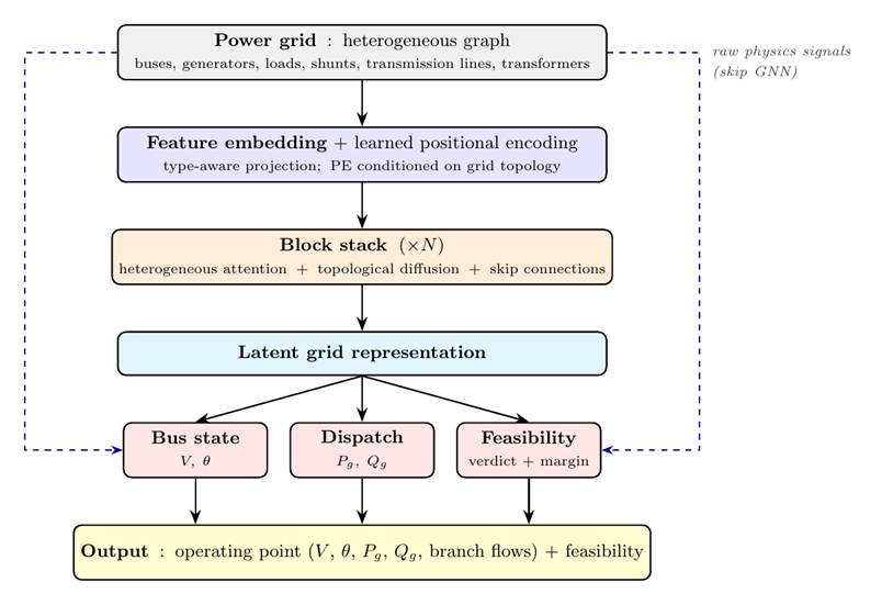 image図 1. GridSFM のアーキテクチャ。バス、発電機、およびブランチの特徴量は共有潜在空間に埋め込まれ、その後、電力網トポロジー上で直接動作するアテンションブロックのスタックによって精緻化されます。出力ヘッドは、この潜在状態を (i) 完全な交流最適潮流(AC-OPF: Alternating Current Optimal Power Flow)運転点、バス電圧および角度、発電機出力配分、ブランチ潮流、および (ii) シナリオごとの実現可能性スコアへとデコードします。
何が可能になるか
電力網の運用や計画における一般的なパターンとして、完全な交流最適潮流(AC-OPF)を用いて少数の手選別されたシナリオを正確に解くことと、物理法則の一部を省略するより高速な近似手法で数千のシナリオを実行することの間で選択を迫られるという状況があります。例えば、一般的に使用されるツールとして直流最適潮流(DC-OPF)近似が挙げられます。これは電圧の実効値を平坦、角度差を微小とし、無効電力および損失を無視する線形化されたバージョンです。この DC 近似は、完全な AC 解析では数分から数時間かかる計算を数秒で解決するため、現在の多くの事故スクリーニング、市場清算の前段階、および計画スウィープが DC 近似上で実行されています。その代償は現実的なものです:DC 近似は電圧および無効制約を完全に無視しており、ストレスのかかるシナリオでは AC の最適解から dispatch コストが 10% を超えて外れる可能性があります(テストベンチマークにおける最悪ケースの電力網では 20% を超える場合もあります)。
必ず JSON 形式で返してください。translation フィールドのみ。他のフィールド (technical_terms 等) は一切追加しないこと — 余計なフィールドを書こうとして本文翻訳がトークン上限で打ち切られる事故を防ぐため:
{"translation": "翻訳全文"}
GridSFM は、高速近似が必要な場面で DC 近似の代替として設計されており、新しいトポロジーごとに再学習を必要とする既存の AC-OPF(交流最適潮流)ニューラルサロゲートとは異なり、対応するサイズ範囲内のグリッド間で再学習なしに一般化するため、DC 近似と同様に普遍的に導入可能です。特に DC-OPF と比較すると、GridSFM には以下の 3 つの具体的な利点があります:
単独運用コストにおける精度クラスは DC 近似と同等です。GridSFM と DC は、シナリオごとのコストギャップ分布(§2 / Figure 6)において同じ範囲に収まり、互いに補完的な失敗モードを示します。DC は、損失なし・無反応性の線形化が構造的に誤りとなるグリッドで失敗し、GridSFM はその学習分布外のグリッドで失敗します。この二つの限界は直交する軸上で解消されます。DC の性能上限は線形化によって固定されていますが、GridSFM の性能の裾野は追加の学習データによって拡大していきます。
完全な AC ソルバーに比べて 1,000 倍高速で、推論ステップにおいては DC 近似よりも約 100 倍高速です。この速度であれば、単一の汎用 GPU で数分以内に数千件の事故(例:送電線や発電機の停電)をシミュレーションすることも可能です。
これは線形近似ではなく、実際の AC 運転点です。GridSFM は電圧と無効電力を生成するため、その予測結果は従来の数値ソルバーに AC ウォームスタートとして引き渡すことができ、DC 近似では実現できないワークフローを開きます。
- 実行可能性スクリーニング:ストレススコアによるトリアージ
あるシナリオにおいて、すべての制約を同時に満たすような運用計画が存在しない場合、そのシナリオは実行不可能となります。具体的には、要求された負荷が電圧範囲や熱的限界、あるいは発電機の容量の制約内で供給できない状態です。運用上、実行不可能性は最も重大な失敗信号であり、要求された運転条件を全く実現できず、対応策として介入(負荷切り捨て、再配分、熱的限界の緩和など)が必要となります。また、これはスクリーニングにおいて最もコストがかかるシナリオのクラスでもあります。なぜなら、ソルバーは非収束に達するまで反復計算を行うことで初めて実行不可能であることを認識するため、各実行不可能ケースには通常、実行可能なケースよりも長い完全なソルバー実行が要されるからです。したがって、実行不可能なものを特定するために数千もの事故やストレスケースを網羅的に調べることは、あらゆる計画ワークフローにおける最悪の場合の計算リソースを大きく消費する作業の一つです。
GridSFM は、各シナリオごとのストレススコアをディスパッチヘッドと共同で訓練することでこの課題に対処します。このスコアは、各グリッド上の 3 つのクラス(シナリオ)に対して評価されます。具体的には、「real-feas」は AC-OPF ソルバーが正常に収束したシナリオ(つまり、実際に実行可能な運転点)、"real-infeas" はソルバーが収束に失敗したシナリオ(実際に実行不可能な運転点)、そして "synth-infeas" は特定の制約(電圧絞り込み、熱的ボトルネック、角度制限、または直流熱的混雑)を違反するように意図的に摂動された実行可能なベースポイントです。54 グリッドのテストシナリオ全体を通じて、ストレススコアのグリッドごとの二値精度はクラス間で広く均一です:real-feas(緑色)の平均は 94.5%、real-infeas(赤色)の平均は 96.1%、synth-infeas(橙色)の平均は 90.4% です。ほとんどのグリッドはこれらの平均値から数ポイント以内にクラスタリングしており、80% を下回る外れ値は、以下のコストギャップ分析で示される同じ困難なグリッドです。
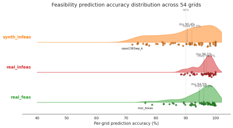 image図 2. 54 グリッドのテストシナリオ全体における GridSM のグリッドごとの実行可能性予測精度をクラス別(real-feas, real-infeas, synth_infesible)に分解した結果。塗りつぶされた KDE と各グリッドのドットを表示し、平均値(–)と中央値(:)を薄い破線で示しています。3 つの分布は大きく重なっており、モデルの品質はクラス間で広く均一ですが、構造的に困難なグリッドによる小さな失敗する尾部が存在します。
ケーススタディに踏み込んでみましょう。代表例となる単一のグリッド、すなわちテキサス2kの夏ピーク時グリッド(新しいタブで開く)にズームインし、学習された表現が予測において実現可能性とROCをどのように分離するかを示します。
表現。図3は、各テキサス2kシナリオに対するモデルの学習された表現を可視化しています。グラフごとの表現(128次元)を、シナリオクラスを実行可能、実行不能、合成不可能に最大限に分離するように選択した2つの軸(LD1, LD2)上に投影します。128次元を2次元に圧縮する過程で情報の損失は避けられないため、この視覚化では見かけ上の重なりが強調されてしまいます。ここでは混在して見えるクラスでも、モデルが実際に使用する完全な128次元空間内では明確に分離可能である可能性があります。着色された雲は各クラスのグラフが集中している領域を示し、各雲の中心にある十字はそのクラスの重心(クラスタ centroid)を表します。これはそのクラスのすべてのグラフの平均位置です。重心同士が大きく離れていることは、モデルがそれらのクラスを明確に区別できていることを意味します。一方、2つの着色された雲が重なっている領域では、異なるラベルを持つグラフに対してモデルが類似した埋め込み(embedding)を生成していることになります。
図 3. Texas2k シナリオにおけるグリッド埋め込みの線形判別分析投影。実在する実行可能ケース(緑)、実在する非実行可能ケース(赤)、および合成された非実行可能ケース(オレンジ)を、クラス間分離を最大化するように選択した 2 つの軸(LD1, LD2)上に投影しています。十字印は各クラスの重心を示し、着色された雲状の領域は各クラスが集中する範囲を表します。雲同士の重なりは、モデルがそれらのクラスに属するグラフに対して類似した埋め込みを生成していることを意味しますが、完全な 128 次元空間では、図示されていない方向に沿ってモデルがこれらを分離できている可能性があります。
運用と ROC(受容者作動特性)。スコア自体は連続値であり、ランキング補正済みです。図 4 はテスト混合データにおける ROC を示しており、曲線下面積(AUC)は 0.986 です。自然な運用点において、このスコアをバイナリ分類器として閾値処理すると、精度は 95.5% となります。その閾値におけるモード別検出性能は、制約条件を明確に限界を超えさせる 3 つの摂動モードすべてで 99〜100% です。
図 4. GridSFM の実行可能性に対するストレスコアの ROC 曲線(Texas2k 夏ピークテスト混合データ:実在する実行可能ケース + ソルバーがラベル付けした非実行可能ケース + 制約条件を限界を超えさせる合成摂動モード)。曲線下面積は 0.986、自然な運用点におけるバイナリ精度は 95.5% です。このスコアはランキング用に補正されていますが、バイナリのカットオフ線をどこに引くかはオペレータの判断次第です。
選別カットオフ。ルーティングシナリオをアクションバケットに振り分ける際、図 5 は各集団におけるストレススコアの分布を示しています。オペレーターは自らのワークフローに合致するカットオフを選択します:非常に自信のある実行可能ケースは示唆的dispatch(ディスパッチ)へ通過し、非常に自信のあるストレス状態のシナリオはエンジニアリングレビューのためにフラグが立てられ、境界線上の中位帯域は検証のためにソルバーへ送られます。このカットオフは、ソルバーの予算とスクリーニングの見落とし率とのバランスを設定するものです。
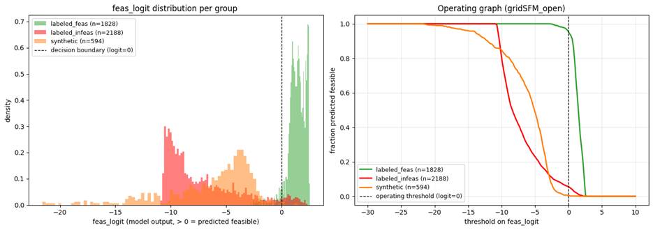 image図 5. 同じ Texas2k テストシナリオにおけるモデルの実行可能性ロジットの分布を、集団別に分割した結果:実在する実行可能ケース(緑)、実在しない実行不可能ケース(赤)、および合成された実行不可能ケース(オレンジ)。破線の垂直線はロジット=0 となる意思決定境界です。右側のサンプルは実行可能と予測されます。この運用閾値において、実在する実行可能ケースの通過率は 99.5%、実在しない実行不可能ケースの正しく検出される割合は 90.4%、合成された摂動の検出率は 88-100% です。
- GridSFM を高速近似として
GridSFM の予測は、最初から厳密な AC-OPF 解を生成することなく、2 つの用途で使用できます。1 つ目はスタンドアロン型の運用計画とコスト推計として、2 つ目は厳密な数値ソルバーに対する初期推定値(ウォームスタート)としての利用です。両者の性能は、常に以下の 2 つの基準点と比較されます。すなわち、完全な AC-OPF(真の最適解)と DC 近似(確立された高速ベースライン)です。以下に示すすべての数値は、同じテストセットである 54 のグリッドシナリオからなる GridSFM-Open から得られたものです。ソルバーの計算時間は、各シナリオごとにシングルコア CPU ピンニング条件下で測定されています。
スタンドアロン型コスト推計
厳密なソルバーによる往復計算が不要な場合、GridSFM が予測した運用計画を直接コスト計算に用いることができます。テストセットにおいて、GridSFM-Open と DC 近似は同じ精度クラスに属します。平均値(DC 2.80%、GridSFM 3.41%)や中央値(DC 1.81% vs GridSFM 2.23%)が互いに匹敵しており、コストギャップの差が 2 桁にわたるシナリオごとの分布も重なり合っています(図 6)。両者には相互補完的な故障モードがあり、どちらかが他方を完全に支配しているわけではありません。
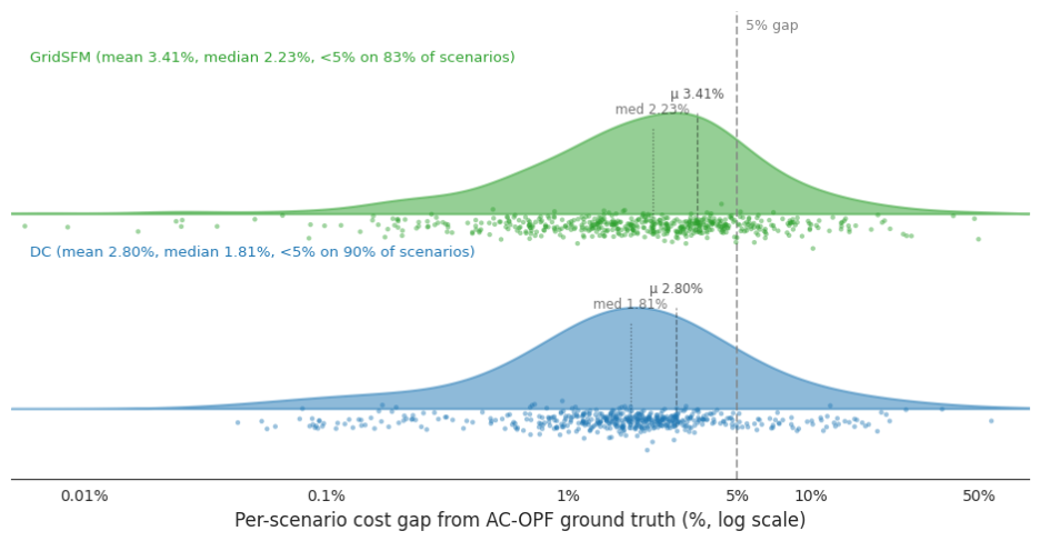 image図 6. AC-OPF 真値からのシナリオ別コストギャップ分布:DC 近似(青)と GridSFM(緑)。GridSFM-Open ベンチマークの 54 グリッド全体にわたる結果。下部には充填されたカーネル密度推定(KDE)および各シナリオごとのプロット点を示し、薄い破線は平均値(–)と中央値(:)を示しています。DC:平均 2.8%、中央値 1.81%
両方の分布は形状において同じように見え、2〜3% のギャップ範囲に単一のピークがあり、シナリオの大部分が 5% 未満で、>25% の範囲に外れ値の小さな尾が伸びています。この外れ値の尾は異なるソースから生じます:DC はその無反応線形化が構造的に誤っているグリッド(case1803_snem および数多くのメッシュ化された送電グリッド)で失敗します;GridSFM の外れ値は、AC-OPF 参照自体が実行可能になるために追加の制約緩和を必要としたいくつかのオープンソース化されたグリッドに集中しており、これらのグリッドにおけるグランドトゥルース目標はノイズが多く、ギャップの一部は参照側の不安定性を反映しています。この二つの限界は直交する軸上で解消されます:DC の上限は線形化によって固定されており、データや計算リソースを増やしても改善しません;GridSFM の尾は、これらのグリッドファミリーに対してよりクリーンな参照ラベルとより多くのトレーニングデータを取得することで解消されます。
したがって、GridSFM の差別化価値は単独のコスト数値ではなく、電圧および無効電力を含む完全な AC 運転点を生成する点にあります。これにより、運用者はグリッドの状態を直接評価できます。これは重要であり、システムの実行可能性と安全性はしばしば電圧および無効電力の限界によって決定されるためです。しかし、DC-OPF ではこれらのいずれも考慮されていません。同時に、この運転点は次章で説明するウォームスタートワークフローも可能にします。
ウォームスタートハンドオフ
AC-OPF ソルバーは、最適性条件が満たされるまで運転点の初期推定値を反復的に改良することで動作し、必要な改良回数は初期推定値が真の最適解にどれだけ近いかによって直接決まります:出発点が悪い場合は数千回の反復が必要になる一方、ほぼ最適な出発点であれば数回で済みます。コールドスタート(フラットスタートとも呼ばれる)では、すべてのバスにおいて電圧大きさを 1.0 p.u.、角度をゼロに設定するため、ソルバーは全量の計算を行います。ウォームスタートはこの汎用的な値をより近い推定値に置き換えることで、ソルバーの収束を高速化します。DC 近似によるウォームスタートでは、まず問題の線形化された DC-OPF バージョンを解き、その解を AC ソルバーのシードとして使用します。一方、GridSFM のウォームスタートではモデルに対して単一の順伝播を実行し、予測された電圧角度と有効電力 Dispatch をソルバーのシードとして使用します。どのウォームスタートももたらせる効果の絶対的な上限を、私たちは GT(ground-truth)上限と呼びます:これはまず高精度で AC-OPF 求解を一度実行して真の最適解を見つけ、その正確な解をウォームスタートのシードとしてソルバーを再実行することによって得られます。これが実用的な求解時間の限界であり、したがって速度向上率の上限となります。
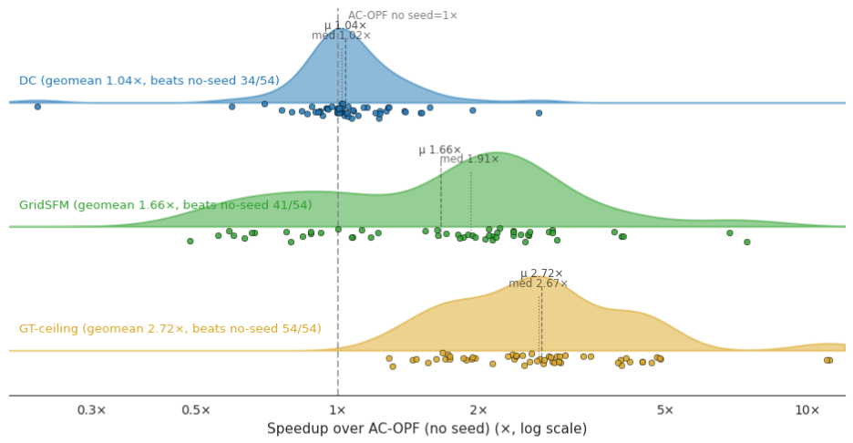
図 7. AC-OPF のコールドスタートに対するウォームスタートの高速化効果(54 系統テストセット全体、対数スケールの x 軸)。GridSFM(緑色)はコールドスタート基準値の直後にきれいに位置し、幾何平均で 1.66 倍の高速化を達成し、54 系統中 41 系統でコールドスタートを上回ります。DC-近似(青色)は幾何平均で 1.04 倍の高速化を達成し、54 系統中 34 系統で性能向上が見られます。GT の上限値(金色、幾何平均 2.72 倍)はウォームスタートの余地に対する上界を示します。各手法の比率は、実行間のタイミングノイズを除去するため、同じ Julia プロセス内で計算されています。
私たちのプロファイルでは、GridSFM のウォームスタートがコールドスタートより 1.66 倍速く、DC-近似のウォームスタートより 1.59 倍速いことが示されました(54 系統のテストシナリオ全体における幾何平均)。また、54 系統中 41 系統で両方のベースラインを上回っています。メッシュ化された送電網(Texas2k 夏のピーク時、case2742_goc)では、コールドスタートに対する個々の系統ごとの最大高速化倍率は 7 倍以上に達します。一方、DC-近似のウォームスタートは、このより広範な系統ミックス全体で平均すると大差ありません(コールドスタートと比較して幾何平均 1.04 倍)。一部の系統では AC 反復回数を節約しますが、他の系統では電圧や無効電力の再構築に時間を費やすことになります。
図 7 に示される GridSFM の分布と GT-上限値の分布(幾何平均 2.72 倍)との差は、次期リリースで目標とする GridSFM の残存無効電力および電圧予測誤差を改善することで縮小可能です。
一般化能力
GridSFM-Open が真のファウンデーションモデルとして機能するかを検証するため、学習時に一度も見たことのないグリッドである OPFData の 6,470 バスケース(6470_rte)で実行しました。これは学習データに含まれるどのグリッドよりも約 1.4 倍大きい規模です。
ゼロショット設定では、予想通り性能は低下します。コスト誤差はインサンプルでは 3.35% ですが、新しいグリッドでは約 14% に増加します。電圧予測は真の変動の約 27% しか捉えられていません。
原文を表示
Microsoft releases a lightweight foundation model that can predict AC optimal power flow in milliseconds, boosting efficiency and unlocking cost savings in grid analysis.
At a glance
Microsoft introduces GridSFM, a small foundation model that approximates AC optimal power flow in milliseconds, unlocking decisions that can directly impact up to $20B/year in congestion losses and 3.4 TWh of renewable curtailment.
Beyond estimating generator dispatch and costs, GridSFM produces full AC system states, giving operators direct visibility into congestion, stability, and overall system health.
It provides a foundation for the community to build advanced power grid simulators and planning tools without recreating data or models from scratch.
Microsoft introduces GridSFM, a small foundation model for solving AC optimal power flow (AC-OPF) problems in transmission power grids. This follows our earlier release of a U.S.-based open transmission-topology dataset that powers GridSFM.
Power grids face increasing strain from surging demand, the need to integrate renewable energy sources, transportation electrification, and extreme weather events. Across all these challenges, the core question is the same: what are the optimal operating points that keep the grid functioning under each new condition?
Answering this requires solving AC optimal power flow (AC‑OPF), a complex, non-convex optimization problem that computes the cheapest generator dispatch (how much each generator produces) that meets demands while respecting power flow physics, voltage limits, thermal constraints, and stability requirements, and underpins core power system operations including reliability, real-time dispatch, market clearing, and contingency analysis. These decisions directly govern outcomes at the scale of up $20 billion per year in congestion costs (opens in new tab) and multi‑terawatt‑hour renewable curtailment (opens in new tab) (lost renewable energy due to congestion), making both economic efficiency and grid reliability highly sensitive to how well these operating points are found. However, AC‑OPF is computationally expensive: power utility scale grid can take up to hours solve, forcing a trade-off between solving a small number of carefully selected scenarios or relying on approximations that ignore critical physics, which can misestimate power flows and binding constraints and lead to suboptimal dispatch and degraded reliability under stressed conditions.
Spotlight: AI-POWERED EXPERIENCE
image
Microsoft research copilot experience
Discover more about research at Microsoft through our AI-powered experience
Start now
Opens in a new tab
To address this limitation, we introduce GridSFM, a single neural network that approximates AC‑OPF in milliseconds across grids ranging from 500 to 80,000 buses. It takes standard AC‑OPF inputs (grid topology, generator and load specifications, transmission line constraints) and produces an operating point and a feasibility verdict (whether the system satisfies all physical and operational constraints). By removing the compute bottleneck, GridSFM makes it possible to evaluate orders of magnitude more scenarios in real time, enabling more informed decisions and shifting grid operations from reactive response to proactive optimization.
In this initial release we offer two tiers:
GridSFM-Open for research-scale grids up to 4,000 buses.
GridSFM-Premier for production-scale systems up to 80,000 buses.
The model is built as a block-structured discrete neural operator (Figure 1), representing each grid as a directed graph, with buses (connection points in the grid) and generators as vertices, and transmission and AC lines as edges. It is trained using both solver supervision, where reference solutions are generated using the AC-OPF solver (IPOPT in PowerModels.jl (opens in new tab)), and physics-based constraints that penalize violations of fundamental physical laws such as Kirchhoff’s voltage and current laws, as well as operating constraints like thermal limits. This enables the model to learn from both feasible and infeasible regimes. Most learning-based AC-OPF surrogates train one model per grid on a narrow distribution (opens in new tab). GridSFM takes the opposite approach: in this release a single model trained across 150+ base grid topologies (network structures) and roughly half a million scenarios spanning varying load profiles, multi-element outages, line-rating derates, voltage-bound tightening, and different generator cost coefficients, so the model is forced to generalize rather than memorize. Across the 54-grid mix test scenarios for GridSFM-Open, our model achieves a median cost gap of 2.23% vs solver ground truth labels (mean 3.41%; warm start seed for traditional numerical solvers, GridSFM-seeded-warm beats cold solve by 1.66× geometric mean across the same test scenarios and beats the industry-standard DC-OPF warm-start by 1.59× geomean (per-grid breakdown and full white-paper analysis to follow). Geometric mean, otherwise known as the multiplicative average, is used here since it is more robust to outliers. Our model also demonstrates the ability to adapt to new grids with just a handful of fine-tune scenarios.
imageFigure 1. GridSFM architecture. Bus, generator, and branch features are embedded into a shared latent space, then refined by a stack of attention blocks operating directly on the grid topology. Output heads decode the latent state into (i) a full AC-OPF operating point, bus voltages and angles, generator dispatch, branch flows, and (ii) a per-scenario feasibility score.
What it enables
A common pattern in grid operations and planning is having to choose between solving a small, hand-picked set of scenarios accurately with full AC-OPF or running thousands of scenarios through a faster approximation that drops parts of the physics. For example, a commonly used tool is the DC-OPF approximation, a linearized version that assumes flat voltage magnitudes and small angle differences and ignores reactive power and losses. DC-approximation solves in seconds what takes full AC minutes to hours, which is why most contingency screens, market-clearing pre-stages, and planning sweeps run on DC-approximation today. The cost is real: DC-approximation ignores voltage and reactive constraints entirely, and its dispatch cost can run >10% off the AC optimum on stressed scenarios (with worst-case grids out past 20% in our test benchmark).
GridSFM is designed as a drop-in alternative to DC-approximation in that fast approximation slot, and unlike most existing AC-OPF neural surrogates, which require a fresh training run for every new topology, GridSFM generalizes across grids in its supported size range without per-topology retraining, so it slots in as universally as DC-approximation. Especially when compared with DC-OPF, GridSFM has three concrete advantages:
Same accuracy class as DC-approximation on standalone dispatch cost. GridSFM and DC fall within the same per-scenario cost-gap distribution (§2 / Figure 6), with complementary failure modes: DC fails on grids where its no-loss / no-reactive linearization is structurally wrong; GridSFM fails on grids outside its training distribution. The two limitations close along orthogonal axes. DC’s ceiling is fixed by the linearization, whereas GridSFM’s tail closes with more training data.
1,000× faster than a full AC solver and approximately 100× faster than DC-approximation at the inference step, fast enough to sweep thousands of contingencies (e.g., line or generator outages) in minutes on a single commodity GPU.
A real AC operating point, not a linear approximation. GridSFM produces voltages and reactive power, so the same prediction can be handed to a traditional numerical solver as an AC warm-start, opening a workflow DC-approximation cannot.
- Feasibility screening: stress-score triage
A scenario is infeasible when no dispatch satisfies all constraints simultaneously: the requested load cannot be served within voltage bounds, thermal limits or generator capacities. Operationally, infeasibility is the most consequential failure signal: the requested operating condition cannot be served at all, and the response is intervention (load shedding, redispatch, relaxing thermal limits). It is also the most expensive class of scenario to screen, because the solver only learns a scenario is infeasible after iterating to non-convergence: each infeasible case costs a full solver run, often longer than a feasible one. Sweeping thousands of contingencies or stress cases to identify the infeasible ones is therefore one of the worst-case budgets in any planning workflow.
GridSFM addresses this with a per-scenario stress score trained jointly with the dispatch head. We evaluate the score on three classes of scenarios on each grid: real-feas are scenarios the AC-OPF solver successfully converged on (i.e., genuinely feasible operating points), real-infeas are scenarios the solver failed to converge on (genuinely infeasible operating points), and synth-infeas are feasible base points we deliberately perturbed to violate a specific constraint (voltage squeeze, thermal bottleneck, angle tightening, or DC-thermal congestion). Across the 54-grid test scenarios, the stress score’s per-grid binary accuracy is broadly uniform across classes: real-feas (green) mean 94.5%, real-infeas (red) mean 96.1%, synth-infeas (orange) mean 90.4%. Most grids cluster within a few points of the means; outliers below 80% are the same hard grids that show up in cost-gap analysis below.
imageFigure 2. GridSM per-grid feasibility prediction accuracy across the 54-grid test scenarios, broken out by class (real-feas, real-infeas, synth_infesible). Filled KDE + per-grid dots, with mean (–) and median (:) light dashed lines. The three distributions overlap heavily, the model’s quality is broadly uniform across classes, with a small failing tail of structurally hard grids.
Drilling into a case study. Let’s zoom into a single representative grid, the Texas2k summer-peak grid (opens in new tab), to show how the learned representation separates feasibility and ROC for predicting.
Representation. Figure 3 visualizes the model’s learned representation of each Texas2k scenario. We project the per-graph representation (128-dimensional) onto two axes (LD1, LD2) chosen to maximally separate the scenario classes: real-feasible, real-infeasible, and synthetic-infeasible. Squeezing 128 dimensions into 2 inevitably loses information, so this view exaggerates apparent overlap: classes that look mixed here may still be cleanly separable in the full 128-dimensional space the model uses. The shaded cloud shows where graphs of each class concentrate, and the cross at the center of each cloud marks the class centroid, the average position of all graphs of that class. Centroids that sit far apart mean the model treats those classes as clearly distinguishable. Where two shaded clouds overlap, the model is producing similar embeddings for graphs with different labels.
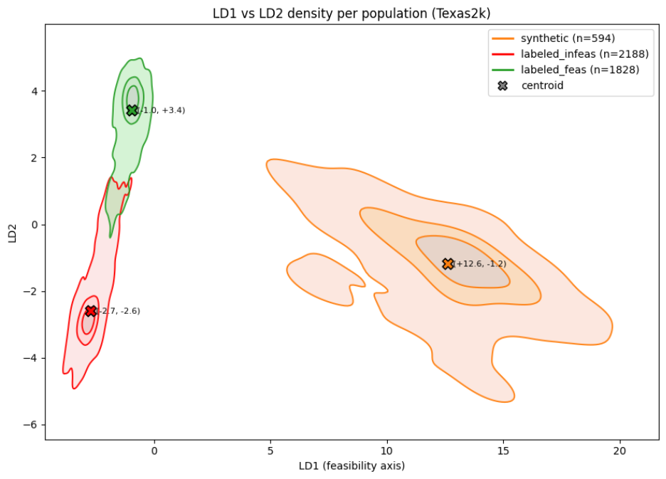 imageFigure 3. Linear discriminant projection of grid embeddings on the Texas2k scenarios. Real feasibles (green), real infeasibles (red), and synthetic infeasibles (orange), projected onto two axes (LD1, LD2) chosen to maximize between-class separation. Crosses mark class centroids; shaded clouds show where each class concentrates. Overlap between clouds means the model produces similar embeddings for graphs in those classes; in the full 128-dimensional space the model may still separate them along directions not shown.
Operation and ROC. The score itself is continuous and ranking-calibrated. Figure 4 shows the ROC over its test mix: AUC = 0.986. At the natural operating point the same score, thresholded as a binary classifier, yields 95.5% accuracy. Per-mode detection at that threshold is 99–100% on the three perturbation modes that drive a constraint cleanly past its limit.
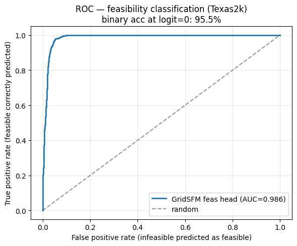 imageFigure 4. ROC curve of the GridSFM stress score for feasibility on the Texas2k summer-peak test mix (real feasibles + solver-labeled infeasibles + synthetic perturbation modes that drive a constraint past its limit). Area under the curve = 0.986, binary accuracy 95.5% at the natural operating point. The score is calibrated for ranking; where to draw the binary cutoff is an operator choice.
Triage cutoff. For routing scenarios into action buckets, Figure 5 shows the stress-score distribution per population. Operators pick the cutoff that matches their workflow: very-confident feasibles pass through to indicative dispatch; very-confident-stressed scenarios are flagged for engineering review; the borderline middle band is sent to the solver for verification. The cutoff sets the balance between solver budget and screening miss-rate.
imageFigure 5. Distribution of the model’s feasibility logit on the same Texas2k test scenarios, split by population: real-feasibles (green), real-infeasibles (red), and synth-infeasibles (orange). The dashed vertical line is the decision boundary where logit=0. Samples to the right are predicted feasible. At this operating threshold, real-feasible pass through at 99.5%, real-infeas are correctly flagged at 90.4%, and the synthetic perturbation are caught at 88-100%.
- GridSFM as a fast approximation
GridSFM’s prediction can be used in two ways without producing an exact AC-OPF solution from scratch: as a standalone dispatch and cost estimate, or as the initial guess (warm-start) for an exact numerical solver. We compare both against the same two reference points throughout: full AC-OPF (the ground-truth optimum) and DC-approximation (the established fast baseline). All numbers below come from the same test set of 54 grids scenarios GridSFM-Open, with solver solve_time measured per scenario under single-core CPU pinning.
Standalone cost estimate
When an exact solver round-trip is not required, GridSFM’s predicted dispatch can be costed directly. In our test set, GridSFM-Open and DC-approximation fall in the same accuracy class: comparable means (DC 2.80%, GridSFM 3.41%), comparable medians (DC 1.81% vs GridSFM 2.23%), and overlapping per-scenario distributions across two decades of cost gap (Figure 6). They have complementary failure modes rather than one dominating the other.
imageFigure 6. Per-scenario cost-gap distribution from AC-OPF ground truth: DC-approximation (blue) and GridSFM (green) across the 54-grid GridSFM-Open benchmark. Filled KDE + per-scenario dots underneath; light dashed lines mark mean (–) and median (:). DC: mean 2.8%, median 1.81%,
Both distributions look the same in shape: a single peak in the 2–3% gap range, with the bulk of scenarios under 5% and a small tail of outliers extending out into the >25% range. The outlier tails come from different sources: DC fails on grids where its no-reactive linearization is structurally wrong (case1803_snem and a handful of meshed transmission grids); GridSFM’s outliers are concentrated on a few of our open sourced grids whose AC-OPF reference itself required additional constraint relaxation to become feasible (opens in new tab), so the ground-truth target on those grids is noisier and the gap partly reflects reference-side instability. The two limitations close along orthogonal axes: DC’s ceiling is fixed by the linearization and does not improve with more data or compute; GridSFM’s tail closes with cleaner reference labels and more training data on those grid families.
The differentiating value of GridSFM is therefore not the standalone cost number, but that GridSFM produces a full AC operating point including voltages and reactive power. This allows operators to directly assess the state of the grid. This is important since the feasibility and security of a system is often determined by the voltage and reactive power limits, but neither are considered in DC-OPF. At the same time, the operating point also enables the warm-start workflow, as we describe next.
Warm-start handoff
An AC-OPF solver works by iteratively refining an initial guess of the operating point until the optimality conditions are satisfied, and the number of refinement iterations it needs depends directly on how close the initial guess starts to the true optimum: a poor starting point can require thousands of iterations, a near-optimal one only a couple. A cold start (also known as a flat start) sets voltage magnitude to 1.0 per unit and angle to zero on every bus, so the solver does the full amount of work. A warm start replaces that generic value with a closer estimate to make the solver converge faster. DC-approximation warm-start solves the linearized DC-OPF version of the problem first and seeds the AC solver with that solution. Whereas, GridSFM warm-start runs a single forward pass through the model and seeds the solver with its predicted voltage angles and active dispatch. The absolute ceiling on how much any warm-start can help is what we call the GT (ground-truth) ceiling: we run the full AC-OPF solve once at high precision to find the true optimum, then re-run the solver with that exact solution as the warm start seed. This is the practical limit on solving time and therefore the ceiling on speedup.
 imageFigure 7. Warm-start speedup over AC-OPF cold start, across the 54-grid test set (log-scale x axis). GridSFM (green, sits cleanly right of the cold-start reference) achieves a geomean speedup of 1.66×, and outperforms cold start on 41 of 54 grids ; DC-approximation (blue) achieves a geomean speedup of 1.04× and improves performance on 34 of 54 grids; the GT ceiling (gold, geomean 2.72×) is the upper bound on warm-start headroom. Each method’s ratio is computed within the same Julia process to remove cross-run timing noise.
Our profile showed that GridSFM warm-start is 1.66× faster than cold start and 1.59× faster than DC-approximation warm-start (geometric means across the 54 grids test scenarios) and is faster than both baselines on 41 of 54 grids. The largest per-grid speedups exceed 7× over cold on the meshed transmission grids (Texas2k summer-peak, case2742_goc). DC-approximation warm-start, by contrast, is a wash on average across this broader grid mix (geomean 1.04× vs cold), DC saves on AC iterations on some grids and spends them rebuilding voltage/reactive on others.
The gap between the GridSFM distribution in Figure 7 and the GT-ceiling distribution (2.72× geomean) can be closed by improving GridSFM’s residual reactive-power and voltage prediction error, both targeted by the next release.
Generalization
We tested whether GridSFM-Open acts like a true foundation model by running it on a grid it had never seen before: the 6,470-bus case6470_rte from OPFData (opens in new tab), about 1.4× larger than any grid in training.
In a zero-shot setting, performance drops as expected. Cost error increases from 3.35% in-sample to about 14% on the new grid. Voltage predictions capture only about 27% of the true varia
関連記事
今日のまとめ
AI日報で今日の重要ニュースをまとめ読み