Tritonにおけるインライン要素別アセンブリによる命令レベルの制御

![image](https://storage.ghost.io/c/0e/15/0e15ee8a-bd95-4b71-9258-950f77f4d196/content/images/2026/02/ff4.png) Triton は、Python で高速な GPU カーネルを書くことを欺瞞的に容易にする DSL（ドメイン固有言語）です。これは、純粋な GPU カーネルをゼロから書く際の微妙なニュアンス、つまり手動のメモリ階層処理、同期、低レベルな起動設定などを抽象化しつつも、高度に最適化された GPU コードを生成します。 しかし、Triton カーネルが生成しない可能性のあるデバイス固有のアセンブリ命令（ビットのパッキングや、特殊/高速な命令の使用など）に対して正確な制御を行いたい瞬間に、壁にぶつかります。この壁は通常、より低いレベルへ降りて、任意のアセンブリ命令を書き込める場所へと人々を導く地点です。 この壁を克服するために、Triton は中間的な API を提供しています：インライン要素別アセンブリ（Inline Elementwise ASM） この記事では、Python の快適な環境から一度も離れることなく、どのようにして Triton で要素別 GPU アセンブリ命令を注入できるか、そしてこのアプローチが実際に価値があるのはどのような場合かを紹介します。まず、Triton カーネルが実際には何にコンパイルされるのかを簡単に理解しましょう。なお、本記事は NVIDIA GPU に焦点を当てており、デバイス固有のアセンブリも PTX と呼ばれます。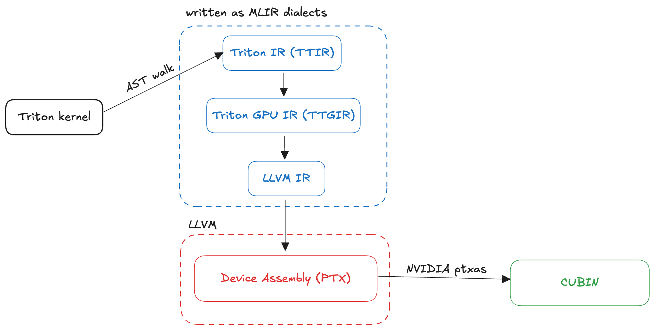 Python から PTX へ Triton は、多くの lowering ステージを経て Python からデバイス固有のアセンブリへと変換されます。Kapil Sharma による素晴らしい記事が、Triton カーネルのコンパイル中に実際に何が起こるかを要約しています： Python カーネルは、テンソルとカーネルのセマンティクスを表す高レベルな Triton IR へパースされます。 この IR は、MLIR ダイアレクト（Triton -> TritonGPU -> TritonNVIDIAGPU）を通じて段階的に低レベル化され、タイル処理、ベクトル化、共通部分式除去 (CSE)、定数畳み込みといったドメイン固有の最適化が適用されます。 最適化された Triton IR は LLVM IR へさらに低レベル化され、追加のコンパイラ最適化を可能にします。 LLVM IR は、NVIDIA の GPU 中間表現である PTX へと翻訳されます。 PTX は NVIDIA のツールチェーンによって JIT コンパイルされ CUBIN となり、GPU で実行されます。 以下の画像は、Triton カーネルのコンパイル中に何が起こるかの視覚的な表現を示しています： ![image](https://storage.googleapis.com/falserverless/example_inputs/triton_lowering_trans.png) 次に、Triton カーネル内で単一の要素ごとの PTX 命令を注入する例を見てみましょう。 例 1: 単一命令 (rcp) Triton は、与えられた引数に対して要素ごとに動作する PTX 命令を注入できる inline_elementwise_asm 関数を提供しています。この関数のシグネチャは以下の通りです： triton.language.inline_asm_elementwise(asm: str, constraints: str, args: Sequence, dtype: dtype | Sequence[dtype], is_pure: bool, pack: int, _semantic=None) このブログ記事では、この関数が受け取る引数について順に説明していきますが、まずは以下の例に焦点を当てましょう。 仮に、形状 (M, N) の 2 つの float32 行列 A と B が与えられており、同じ形状を持つ別の行列 C を計算したいとします。ここで、C は次のように定義されます： ci = ai / bi この演算は、float32 データ型に対して Triton で容易に利用可能です。しかし、別の方法でも結果を計算できます： ci = ai * (1 / bi) ここで (1 / bi) は、bi 値の逆数（reciprocal）です。これを覚えておいてください。 この演算に対する、インライン PTX を含まない通常の Triton カーネルは、以下のようなものになります： @triton.jit def _kernel( a_ptr, b_ptr, c_ptr, N, BLOCK_SIZE: tl.constexpr = 1024 ): pid = tl.program_id(0) offs = pid * BLOCK_SIZE + tl.arange(0, BLOCK_SIZE) mask = offs < N a = tl.load(a_ptr + offs, mask=mask, other=0.0) b = tl.load(b_ptr + offs, mask=mask, other=1.0) c = a / b tl.store(c_ptr + offs, c, mask=mask) このカーネルに対するホスト関数は以下のようになります： def div(a: torch.Tensor, b: torch.Tensor, version=1): numel = a.numel() out = torch.empty_like(a) grid = lambda meta: (triton.cdiv(numel, meta['BLOCK_SIZE']), ) K = _kernel[grid](a, b, out, numel, BLOCK_SIZE=1024) return out, K このカーネルの Triton によってコンパイルされた PTX を、K.asm['ptx'] をファイルにダンプすることで確認できます。そうすると、Triton が PTX で ai / bi を計算するために以下の命令を使用していることがわかります： div.full.f32 d, a, b; ここで、値 ai は 32 ビットレジスタ a に格納され、値 bi は 32 ビットレジスタ b に格納され、結果は d に格納されます。 PTX のドキュメントを確認すると、与えられた float32 値の高速な近似逆数（reciprocal）を計算する命令が見つかります： rcp.approx{.ftz}.f32 d, a; したがって、必要であれば、bi 値の高速な近似逆数を計算し、その結果を ai 値に掛けることができます。これを行うには、カーネルを以下のように更新する必要があります: @triton.jit def _kernel( a_ptr, b_ptr, c_ptr, N, BLOCK_SIZE: tl.constexpr = 1024 ): pid = tl.program_id(0) offs = pid * BLOCK_SIZE + tl.arange(0, BLOCK_SIZE) mask = offs < N a = tl.load(a_ptr + offs, mask=mask, other=0.0) b = tl.load(b_ptr + offs, mask=mask, other=1.0) (multiplier,) = tl.inline_asm_elementwise( asm="rcp.approx.ftz.f32 $0, $1;", constraints="=r,r", args=[b], dtype=[tl.float32], is_pure=True, pack=1 ) c = a * multiplier tl.store(c_ptr + offs, c, mask=mask) 本質的には、これはトリトンテンソルの要素に対するマップ演算であり、その関数はインライン PTX です。 asm: これはテンソルの要素に対して使用される文字列命令です。要素を 32 ビットレジスタとしてアクセスするには、プレースホルダーの $0, $1, $2 などを使用できます。 constraints: これは、入力および出力テンソルとデータ型の数に基づいて、トリトンに出力および入力レジスタの数を伝える文字列です。より詳しく理解するためには、ASM LLVM フォーマットドキュメントをご覧ください。出力レジスタは =r で識別され、入力レジスタは r です。 args: 値がインラインアセンブリブロックへ 32 ビットレジスタとして渡される入力トリトンテンソルです。 dtype: 返されるテンソルの要素型です。出力レジスタとその dtype を正しく設定して誤った結果を避けることはプログラマの責任です。 is_pure: true の場合、Triton コンパイラは ASM ブロックに副作用がないと仮定し、インライン ASM はそのまま動作します。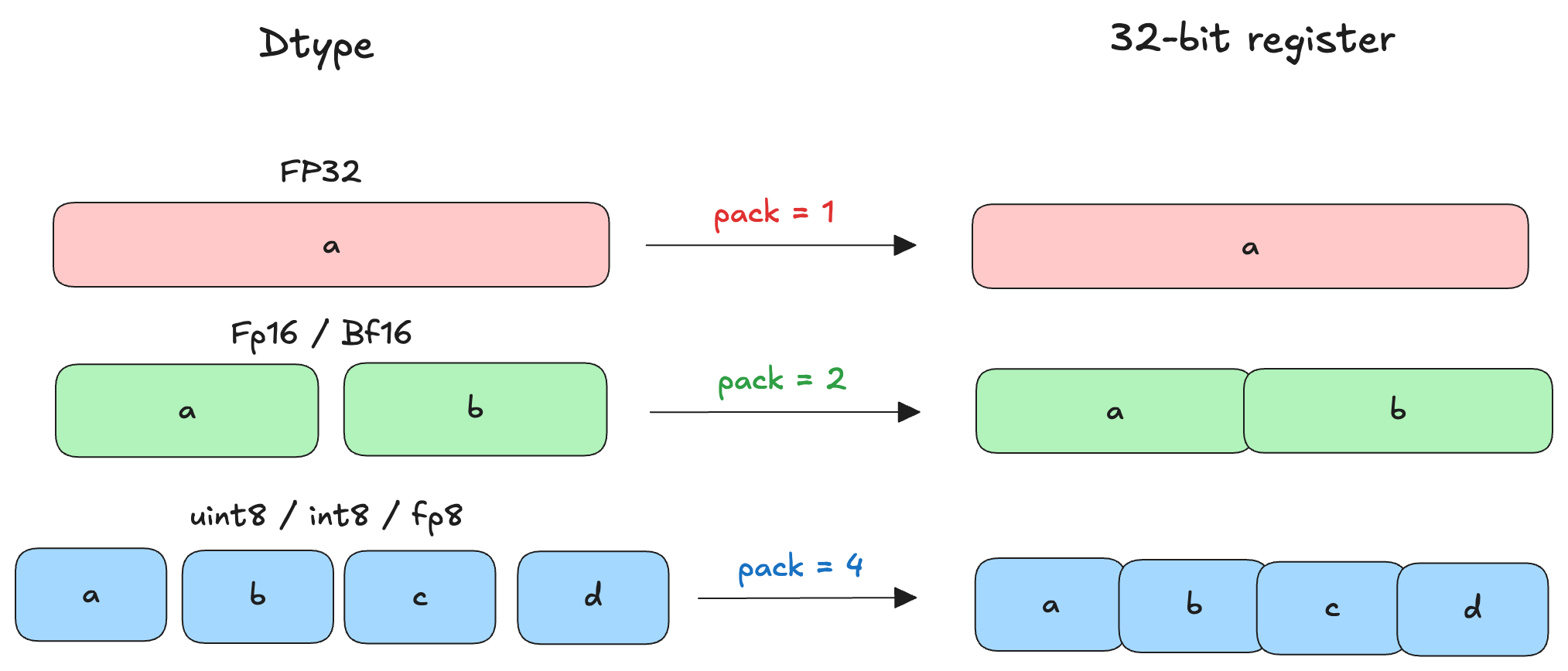 pack: インライン ASM の各呼び出しでは、一度にパックされた要素が処理されます。ブロックがどの入力セットを受け取るかは指定されていません。4 バイト（32 ビット）未満のサイズの要素は、4 バイト（32 ビット）レジスタにパッキングされます。 この例では float32 dtype のみを扱っているため、パッキングは不要であり、一度に 1 つの要素のみを処理します。 両方のバージョンを実行すると出力に違いは見られませんが、Triton が生成した PTX を検査してみると以下のようになります： version 1 で生成された PTX div.full.f32 %r33, %r1, %r17; div.full.f32 %r34, %r2, %r18; div.full.f32 %r35, %r3, %r19; div.full.f32 %r36, %r4, %r20; div.full.f32 %r37, %r9, %r25; div.full.f32 %r38, %r10, %r26; div.full.f32 %r39, %r11, %r27; div.full.f32 %r40, %r12, %r28; 実行時間：0.12382 ms version 2 で生成された PTX rcp.approx.ftz.f32 %r33, %r34; rcp.approx.ftz.f32 %r35, %r36; rcp.approx.ftz.f32 %r37, %r38; rcp.approx.ftz.f32 %r39, %r40; rcp.approx.ftz.f32 %r41, %r42; rcp.approx.ftz.f32 %r43, %r44; rcp.approx.ftz.f32 %r45, %r46; rcp.approx.ftz.f32 %r47, %r48; mul.f32 %r49, %r33, %r1; mul.f32 %r50, %r35, %r2; mul.f32 %r51, %r37, %r3; mul.f32 %r52, %r39, %r4; mul.f32 %r53, %r41, %r9; mul.f32 %r54, %r43, %r10; mul.f32 %r55, %r45, %r11; mul.f32 %r56, %r47, %r12; 実行時間：0.12375 ミリ秒 実際、2 番目のバージョンの方が 1 番目のバージョンよりわずかに高速です！それ以外にも、ビットパッキングや特殊命令などを操作する必要がある場合、通常の Triton に比べて要素ごとの PTX（Program Thread eXecution）を注入することで、はるかに多くの柔軟性が得られます。 例 2：パッキングと複数の命令 形状が (N,) の float16 配列 A と B が 2 つあり、C と D を以下のように計算したいとします。 ci = ai * bi + 1.0 ci = clamp(ci, 0.0, 6.0) di = ci * ci ここでデータ型が float16 の場合、要素ごとのアセンブリ関数を使用して一度に 2 つの要素を処理できます。Triton は自動的に 32 ビットレジスタ内に 2 つの float16 値をパッキングします。これに加えて、C と D を計算するために以下の f16x2 PTX 命令を使用できます。 fma.rnd{.ftz}{.sat}.f16x2 d, a, b, c; max{.ftz}{.NaN}{.xorsign.abs}.f16x2 d, a, b; mul{.rnd}{.ftz}{.sat}.f16x2 d, a, b; 通常のカーネルと PTX を注入したカーネルは以下のようになります。 @triton.jit def kernel_fp16_normal(A, B, C, D, BLOCK: tl.constexpr): offs = tl.program_id(0) * BLOCK + tl.arange(0, BLOCK) a = tl.load(A + offs) b = tl.load(B + offs) y = a * b + 1.0 y = tl.clamp(y, 0.0, 6.0) tl.store(C + offs, y) tl.store(D + offs, y * y) and, @triton.jit def kernel_fp16_pack2(A, B, C, D, BLOCK: tl.constexpr): offs = tl.program_id(0) * BLOCK + tl.arange(0, BLOCK) a = tl.load(A + offs) b = tl.load(B + offs) (c, d) = tl.inline_asm_elementwise( asm=""" { .reg .b32 tmp ; mov.b32 tmp0, 0x3C003C00; // 1.0 mov.b32 tmp1, 0x00000000; // 0.0 mov.b32 tmp2, 0x46004600; // 6.0 // y = a * b + 1 fma.rn.f16x2 $0, $2, $3, tmp0; // clamp max.f16x2 $0, $0, tmp1; min.f16x2 $0, $0, tmp2; // d = y * y mul.rn.f16x2 $1, $0, $0; } """, constraints="=r,=r,r,r", args=[a, b], dtype=(tl.float16, tl.float16), is_pure=True, pack=2, ) tl.store(C + offs, c) tl.store(D + offs, d) Here, we pass the two Triton tensors as arguments. We use the value of pack as 2 so that Triton can pack two float16 elements in one 32-bit register which we can use with the f16x2 instruction. For the outputs, Triton also unpacks the 32-bit register containing the f16x2 value (32-bit register) to the given output dtype. 以下の画像は、異なるデータ型（dtypes）において要素をパッキングする方法を示しています: ![image](https://storage.googleapis.com/falserverless/example_inputs/pack_asm.png) 出力を比較すると違いは見られませんが、両方のカーネルが達成した実効メモリ帯域幅（GB/s）を見ると、以下のようになります: Normal Triton : 6502.08 GB/s Inline PTX f16x2: 6514.12 GB/s この例では、インライン PTX を使用する二番目のカーネルの方が、最初のカーネルより 12 GB/s 高速であることがわかります！ 上記の簡易な例では、Triton はすでに必要な演算をサポートしています。しかし、ここでは実際の事例を見て、Triton が標準で明示的なサポートを提供していない場合でも PTX 命令を使用できることを理解しましょう。 例 3: Blackwell GPU における NVFP4 量子化 NVFP4 は、形状 (M, N) の与えられた行列 X を FP4 e2m1 データ型へ量子化するブロックスケーリング量子化のレシピです。FP4 の狭い精度を考慮し、量子化誤差を緩和するためにここでは二つのスケールファクタを使用します：グローバルなテンソル全体のスケール（データ型 fp32）と、ローカルなブロックごとのスケール（データ型 FP8 e4m3）です。ここでいうブロックスケールのサイズは 16 で、つまり連続する 16 個の要素が共通のローカルスケーリングファクタを共有します。 形状 (M, N) の行列 X を NVFP4 すなわち fp4 e2m1 データ型へ正確に量子化する方法の詳細には立ち入りませんが、要点は以下の通りです: テンソル全体を通じての絶対最大値（amax_x）を計算する。 グローバルエンコードスケールを (6 × 448) / amax_x として計算し、その逆数を FP32 でグローバルデコードスケールとして保存します。 テンソルを Tensor Core の粒度に一致する連続ブロックに分割します。 各ブロックに対して、ブロック絶対最大値 (amax_b) を計算し、ローカルデコードスケールを amax_b / 6 として算出します。 ローカルデコードスケールにグローバルエンコードスケールを乗算し、偶数への丸めを用いて FP8 (E4M3) に量子化します。 量子化された FP8 デコードスケールの逆数を適用し、グローバルデコードスケールを乗じることで、有効なローカルエンコードスケールを復元します。 ブロック内の各値をローカルエンコードスケールでスケーリングし、FP4 に量子化して保存します。GEMM には FP4 の値とともに、FP8 のローカルデコードスケールと FP32 のグローバルデコードスケールも併せて格納します。 ここで重要なのは、この量子化レシピを PyTorch で記述する場合、ビット操作やビットパッキング演算を工夫して行う必要があるということです。以下の疑似コードは、その関数がどのような見た目になるかを示しています: function QUANT_NVFP4(x): assert last_dim(x) % 16 == 0 x_blocks <- reshape x into (..., N/16, 16) as FP32 if global_scale not provided: global_scale <- (FP4_AMAX * FP8_AMAX) / max(|x_blocks|) s_decb <- max(|x_blocks| over last dim) / FP4_AMAX xs <- clamp(s_decb * global_scale, ±FP8_AMAX) xs <- cast xs to FP8 s_encb <- global_scale / xs s_encb <- expand s_encb to shape (..., N/16, 1) x_scaled <- x_blocks * s_encb xq <- cvt_1xfp32_2xfp4(x_scaled) xs_tiled <- tile_scales_128x4_to_32x16(xs) return xq, xs_tiled, global_scale このヘルパー関数 cvt_1xfp32_2xfp4 は以下のように見えます: thresholds = [ (5.0, 0b0110), (3.5, 0b0101), (2.5, 0b0100), (1.75, 0b0011), (1.25, 0b0010), (0.75, 0b0001), (0.25, 0b0000), ] function cvt_1xfp32_2xfp4(x): sign_bit = MSB(x) x_abs = abs(x) mag_code = 0b0111 for i, (threshold, code) in enumerate(thresholds): if i is even: if x_abs <= threshold: mag_code = code else: if x_abs < threshold: mag_code = code # pack 8 FP4 values into one 32-bit word fp4 = (sign_bit << 3) | mag_code packed = 0 for j in 0..7: packed |= fp4[j] << (4 * j) return reinterpret_as_fp4_dtype(packed) もしこれを Triton カーネルとして記述する場合、カーネル内で Triton テンソルに対してビット操作演算を使用することも可能です。しかし、より賢明な方法として、以下の PTX 命令を使用して float32 を float4 e2m1 に変換することができます: cvt.rn.satfinite{.relu}.e2m1x2.f32 d, a, b; この命令は、2 つの float32 値を 8 ビット（つまり 1 つの uint8 または int8 値）にパッキングされた 2 つの float4 e2m1 値に変換します。この要素ごとの演算を Triton カーネル内で使用することで、複数のビット操作演算を使用する必要がなくなります。実際、Flashinfer や TensorRT-LLM などのライブラリの量子化カーネルでは、float32 値の変換と量子化にこの命令が使用されています。PTX ドキュメントによると: e2m1x2 データ形式への変換を行う際、目的演算子 d は .b8 型となります。2 つの .f32 入力値を .e2m1x2 形式に変換する場合、各入力は指定された形式に変換され、変換後の値は目的演算子 d にパッキングされます。具体的には、入力 a から変換された値が d の上位 4 ビットに格納され、入力 b から変換された値が d の下位 4 ビットに格納されます。 この命令を Triton カーネルで使用する場合の例は以下の通りです： x_e2m1x2 = tl.inline_asm_elementwise( asm=""" { .reg .b8 tmp ; cvt.rn.satfinite.e2m1x2.f32 tmp0, $5, $1; cvt.rn.satfinite.e2m1x2.f32 tmp1, $6, $2; cvt.rn.satfinite.e2m1x2.f32 tmp2, $7, $3; cvt.rn.satfinite.e2m1x2.f32 tmp3, $8, $4; mov.b32 $0, {tmp0, tmp1, tmp2, tmp3}; } """, constraints=( "=r," # 出力 d = $0 "r,r,r,r," # 下位ビット b = $1-$4 "r,r,r,r" # 上位バイト a = $5-$8 ), args=x_blocks_reshaped_split, dtype=tl.int8, is_pure=True, pack=4, ) ここで、Triton は 32 ビットレジスタを扱うため、mov.b32 命令を使用して tmp0-3 で与えられる 4 つの 8 ビット値を 1 つの 32 ビットレジスタにパッキングしています。その後、最終的に出力を int8 データ型に変換します。これが、ここで pack の値が意図的に 4 に設定されている理由です。 100 行未満のコードで書かれたこの注入された PTX Triton カーネルと、2000 行を超える Flashinfer や TensorRT-LLM などのライブラリの量子化カーネルを比較すると、以下の結果が得られます。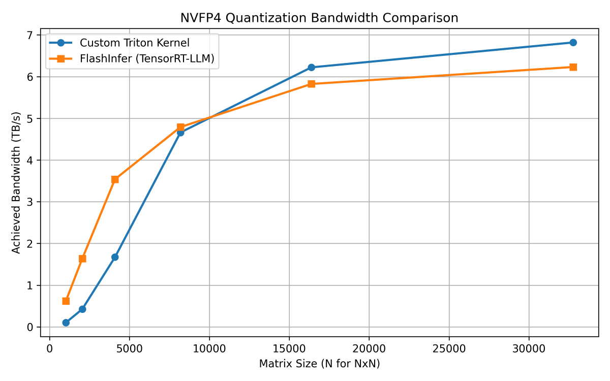 ![image](https://storage.googleapis.com/falserverless/example_inputs/kernel_comparison.png) ご覧の通り、B200 で比較した場合、Triton カーネルは最適化された CUDA カーネルと肩を並べる性能を発揮します。より小さな形状では CUDA カーネルの方が高速ですが、より大きな形状では Triton カーネルが CUDA カーネルを上回り、メモリ帯域幅でほぼ 7 TB/s に達します。 この例は、インライン PTX を用いたわずか 100 行未満の注意深く設計された Triton カーネルによって、最適化された CUDA カーネルと同等の性能、あるいは場合によってはそれを超える性能を、少なくとも GEMM ベースではないワークロードにおいて達成できることを示しています。とても素晴らしい不是吗？ 結びの言葉 Triton におけるインライン要素演算 PTX は、非常に優れたバランス点に到達します。一方では、Python の内部で全てを維持できます：最初に Triton を選んだ理由である生産性、組み合わせ可能性、そして迅速な反復です。他方では、ビットパッキングやベクトル化された f16x2 演算、近似逆数計算、あるいは今日では Triton が直接公開していない cvt.e2m1x2.f32 などの特殊変換操作など、命令選択に対する外科的な制御力を取り戻すことができます。 ただし、これは万能薬ではありません。無視できないいくつかのトレードオフを伴います： 正しさの責任はあなたにあります：レジスタ制約、パッキング係数、データ型は完璧に一致させる必要があります。 デバッグが困難になります：誤った指定された制約は、静かに間違った結果を生み出す可能性があります。 抽象化の漏れが発生します：あなたのカーネルはアーキテクチャ依存となり、ベンダー間や将来の NVIDIA アーキテクチャ間での移植性を確保するには、PTX（Parallel Thread Execution）を見直す必要があるかもしれません。 要素ごとのセマンティクスに制限されます：共有メモリも明示的な同期もワープレベルの制御も利用できません。 最大限の柔軟性が必要で、メモリアーキテクチャ全体への完全な制御やワープレベルの高度な操作などが求められる場合は、CUDA や NVIDIA の CuTe DSL（Domain Specific Language）に降りるのが依然として適切なツールです。実際には、最も効果的なアプローチはハイブリッド型であることが多く、カーネルの大部分をクリーンな Triton で記述し、PTX を本当に重要な箇所にのみ注入します。このように使用することで、インライン要素ごとの PTX は Triton を「高レベル DSL」から、手動最適化された CUDA と競合しつつも Python でコードを書き続けることができる驚くほど鋭い低レベルツールへと変えることができます。 お読みいただきありがとうございます！

Tritonにおけるインライン要素別アセンブリによる命令レベルの制御

背景や根拠まで確認しますか？

このニュースを、実務の判断につなげる

関連記事

調べる

選ぶ

サイト