NVIDIA Blackwell を用いた Amazon SageMaker AI でのモデル学習の最適化
AWS は Amazon SageMaker AI で NVIDIA Blackwell ベースの P6-B200 インスタンスを一般提供し、大規模モデルのトレーニングにおけるメモリ制約や通信オーバーヘッドを低減する具体的な最適化手法を提示した。
キーポイント
P6-B200 インスタンスの可用性と柔軟な利用
Amazon SageMaker AI で NVIDIA Blackwell GPU を搭載した P6-B200 インスタンス(8 GPU)が一般提供され、Flexible Training Plan を通じて予測可能なアクセスとコスト管理が可能になった。
メモリ制約の緩和によるトレーニング効率化
Blackwell の拡張されたメモリ容量により、バッチサイズやシーケンス長を拡大でき、激しいモデル分割(sharding)を減らして通信オーバーヘッドとインフラコストを削減できる。
単一ノードでの大規模モデル実行
適切な精度フォーマットの選択により、従来はマルチノードが必要だった 1B〜64B パラメータのモデルが単一の 8 GPU ノードで実行可能となり、イテレーションサイクルが加速する。
具体的な構成最適化フレームワーク
バッチサイズ、シーケンス長、精度フォーマットの選択、および活性化チェックポイントの戦略的適用に関する実践的な設定ガイドを提供している。
ハイパーパラメータの環境変数化
SageMaker はハイパーパラメータを SM_HP_<NAME> という形式の環境変数としてコンテナに渡すため、スクリプト内でこれらの値を取得してトレーニング設定に適用できます。
Blackwell 対応のカスタム Docker コンテナ構築
AWS Deep Learning Containers をベースに Transformer Engine 2.11 と CUDA ライブラリをインストールしたカスタムコンテナを作成し、FSDP スクリプトを含むことで NVIDIA Blackwell GPU で最適化されたトレーニングを実現します。
CUDA ランタイムの依存関係解決
事前構築済みの flash-attn ウィールが libcudart.so.12 を必要とするため、nvidia-cuda-runtime-cu12 のインストールと LD_LIBRARY_PATH 環境変数の設定が必須です。
影響分析・編集コメントを表示
影響分析
このニュースは、大規模言語モデル(LLM)やマルチモーダルモデルの開発において、ハードウェアの限界に起因するボトルネックを解消し、より安価かつ高速なトレーニング環境を実現する重要な転換点です。AWS と NVIDIA の連携による新インスタンスの提供は、企業の AI 開発コスト構造とスケーラビリティ戦略に直接的な影響を与えるでしょう。
編集コメント
単なるハードウェアのアップデートではなく、大規模モデル開発における「メモリ制約」という根本的な課題を解決する具体的な運用フレームワークが提示されている点が極めて重要です。特に、マルチノードからシングルノードへの移行が可能になることで、インフラ管理の複雑さが劇的に低下し、実務レベルでの即効性が高いと言えます。
NVIDIA Blackwell GPU を用いた Amazon SageMaker AI 上でのモデルトレーニングの最適化は、大規模 AI モデルにとって何が現実的かを根本から変えます。今日、大規模モデルをトレーニングしている場合、おそらく以下のようなお馴染みの制約に直面しているでしょう:GPU メモリによって制限されるバッチサイズ、メモリ不足エラーを防ぐために短く切られたシーケンス長、スケールする際に通信オーバーヘッドを追加するモデルのシャード化です。Blackwell の拡張されたメモリと新しい精度フォーマットは、これらの制約を直接的に軽減します。8 枚の Blackwell GPU を搭載した P6-B200 インスタンスは Amazon SageMaker AI でトレーニングジョブとして利用可能であり、予測可能なアクセス、コスト管理、自動化されたリソース管理を提供する Flexible Training Plan を用いてキャパシティを予約できます。Amazon SageMaker AI のトレーニングジョブでは、基盤となるコンピューティングインフラストラクチャとリソースの自動プロビジョニングおよび管理を行うことで、大規模な ML モデルのトレーニングが可能となり、インフラストラクチャ運用ではなくデータやアルゴリズムに注力することができます。
この投稿では、AWS 上の Blackwell アーキテクチャの性能を最大限に引き出すために、Amazon SageMaker AI でトレーニングジョブを設定する方法をご紹介します。Blackwell の拡張されたメモリを活用するバッチサイズとシーケンス長の選択、モデルサイズ(1B から 64B パラメータ)に応じた適切な精度フォーマットの選定、そして戦略的な活性化チェックポイントの適用方法について学びます。これにより、P6-B200 インスタンス上で分散トレーニングジョブを起動し、トレーニング設定を調整するための実践的なフレームワークが完成します。
適切に設定された Blackwell によるトレーニングジョブでは、積極的なシャード処理を行わずとも大きなバッチサイズを処理でき、通信オーバーヘッドが削減されスループットが向上します。長距離依存関係タスクにおいて、より長いシーケンス長の利用が可能になります。適切な精度フォーマットを採用することで、従来はマルチノード構成が必要だったモデルでも、単一の 8-GPU ノードで実行可能となり、反復サイクルの高速化、ネットワークオーバーヘッドの削減、インフラコストの低減を実現します。
NVIDIA Blackwell の理解
トレーニングジョブを設定する前に、Blackwell が以前の GPU 世代と何が異なるのかを理解しておくことが役立ちます。Blackwell のデュアルチップアーキテクチャと第 5 世代 Tensor Cores は、マルチ GPU トレーニングにおいて即座に測定可能な向上をもたらします。NVLink 5 インターコネクトは、双方向の GPU から GPU への帯域幅を最大 1.8 TB/s 提供し、B200 の大容量 HBM と高いメモリ帯域幅は、大規模バッチ、長いシーケンス、および分散トレーニングワークロードにおけるメモリの圧力を軽減するのに役立ちます。
本記事の例では、1B から 64B パラメータまでのトランスフォーマーモデルを用いたシングルノード 8 GPU トレーニングを使用します。トレーニング設定には、PyTorch Fully Sharded Data Parallel (FSDP) が使用されており、これはモデルパラメータ、勾配、オプティマイザ状態を GPU にシャードして、単一 GPU メモリを超える大規模なモデルをトレーニングするための分散トレーニング技術です。結果は、異なるアプローチが最適な結果をもたらすタイミングを示すために、バッチサイズ、シーケンス長、および精度フォーマットを変えた複数の構成をカバーしています。
メモリ管理
Blackwell の拡張されたメモリ(B200 で 180 GB、B300 で 268 GB)は、より大きなバッチサイズ、簡素化されたモデルシャード、および長いシーケンス長の 3 つの領域で最適化する余地を与えてくれます。
- より大きなバッチサイズは、GPU 間での勾配同期ステップ数を減らし、全体のスループットを向上させます。
- GPU あたりのメモリ容量が増えることでモデルのシャード化が簡素化され、一部のモデルでは並列度の低下や並列処理の完全な排除が可能になります。シャード数が減れば、GPU 間通信のオーバーヘッドも削減されます。
- より長いシーケンス長により、モデルは1回のパスでより多くのコンテキストを処理できるようになり、これは長期依存関係を持つタスクにおいて極めて重要です。
スループットが主目的であればバッチサイズの調整から始めましょう。通信オーバーヘッドがボトルネックとなっている場合はシャード化の簡素化を優先してください。タスクに長期的な文脈が必要であればシーケンス長の最適化を最優先します。バッチサイズとシーケンス長の両方はメモリ消費量を増加させるため、効果的なバランスを見つけることが重要です。
アクティベーションチェックポイント(activation checkpointing)は、メモリの使用量と計算処理のバランスを取るのに役立ちます。これは、逆伝播時に中間活性化値を保存する代わりに再計算することで GPU メモリ使用量を削減し、その代償として計算時間が増加します(モデルアーキテクチャにもよりますが通常 10〜30% のオーバーヘッドが発生します)。解放されたメモリは、より大きなバッチサイズや長いシーケンス長のために再投資できます。計算オーバーヘッドはワークロードによって異なるため、チェックポイント化を採用する前に、具体的な構成でベンチマークを行い、トレードオフを理解しておく必要があります。
例えば、図 1 では、8K シーケンス長において MXFP8 精度を用いた 1B パラメータの LLM に対して、3 つのトレーニング構成を比較しました。アクティベーションチェックポイントなし(バッチサイズ=1)では、スループットは約 6,000 トークン/秒ですが、ピークメモリ使用量は 15.5 GB と高くなります。同じバッチサイズでアクティベーションチェックポイントを有効にすると、中間活性化値が保存される代わりに再計算されるため、メモリ使用量が劇的に 2.3 GB に低下しますが、その再計算オーバーヘッドによりスループットもわずかに低下します。最大のメリットは 3 つ目のバーに見られます:アクティベーションチェックポイントを有効にし、バッチサイズを 16 に引き上げると、解放されたメモリにより大幅に大きなバッチが可能となり、スループットは約 51,000 トークン/秒(ベースラインの約 8 倍)まで向上します。一方、ピークメモリ使用量は 22.8 GB に上昇しますが、これは依然として GPU の制限範囲内に収まっています。
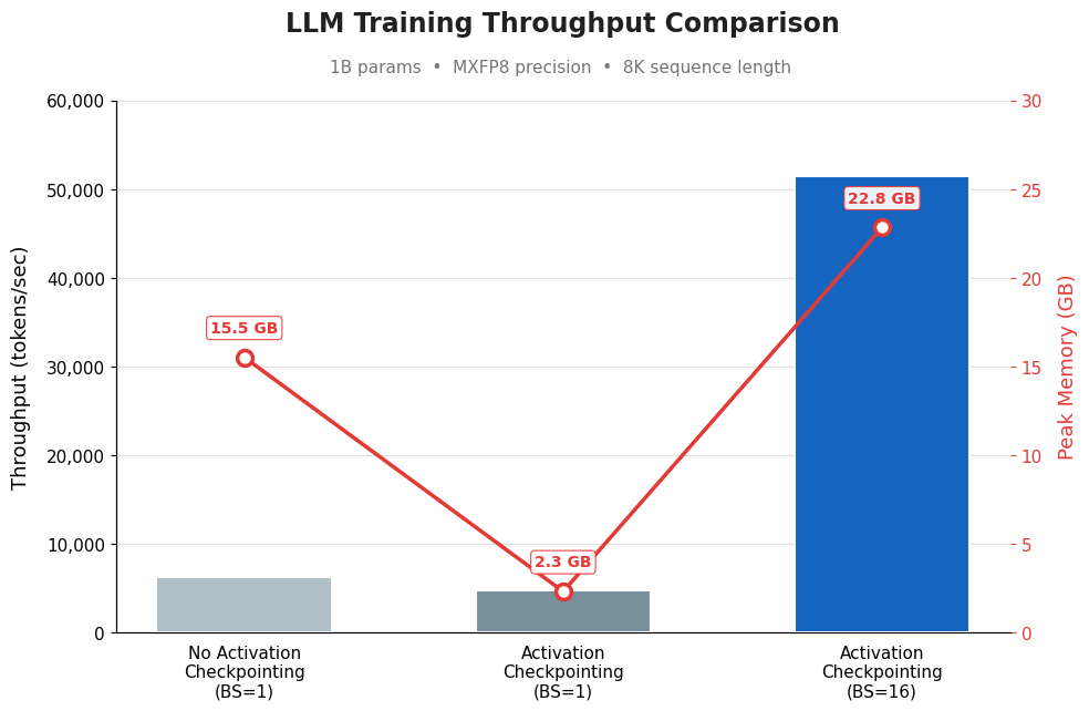
図 1. アクティベーションチェックポイントの有無によるスループットの違い
ワークロードに対してアクティベーションチェックポイントを有効にするべきか判断するには、モデルサイズとメモリ使用量を検討してください:
- 小規模モデル(最大約140億パラメータ):アクティベーションチェックポイントリングは通常不要です。Blackwell の拡張されたメモリにより、ほとんどの小規模モデルはこの機能なしでも余裕を持って動作します。もしこの範囲の上限で実行しておりメモリ圧力に直面している場合、アクティベーションチェックポイントリングを導入すると計算オーバーヘッドが増加する代わりに意味のあるメモリ節約が可能となり、その分をより大きなバッチサイズに再投資できます。
- 大規模モデル(約140億パラメータ以上):このモデルサイズでは、バッチサイズやシーケンス長に応じてメモリ消費量は87GBから171GBの範囲になります。アクティベーションチェックポイントリングなしでは、ほとんどの構成でCUDA のメモリ不足(OOM: Out-Of-Memory)エラーが発生し失敗します。チェックポイントリングを追加すると解放されたメモリによりバッチサイズを十分に増やすことができ、計算オーバーヘッドが増加したにもかかわらずスループットが向上します。大規模モデルにおいては、チェックポイントリングは任意のものではなく、安定したトレーニングのための必須条件です。
Precision formats
Blackwell の第 5 世代 Tensor Cores は、低精度フォーマット(FP8, MXFP8, NVFP4)に対するハードウェアアクセラレーションを提供し、これらは主にスループットの最適化技術であり、メモリ節約を主目的とした手法ではありません。より低い精度を使用することでメモリー帯域幅の要件が軽減され、同時に GPU が 1 サイクルあたりに実行できる演算数が増加します。しかし、デフォルトでは Transformer Engine がオプティマイザ更新用の高精度なプライマリウェイトと量子化されたコピーの両方を保持するため、低精度でのトレーニングは基本的にメモリ使用量に対して中立(メモリーニュートラル)です。つまり、より低い精度フォーマットが直接的にメモリ使用量の低下につながるわけではありません。量子化自体がオーバーヘッド(精度フォーマット間の変換や、メモリ内におけるウェイトの複数コピーの維持)を導入するため、純粋なメリットはモデルサイズと、トレーニングが計算バウンド型かメモリーバウンド型のどちらであるかに依存します。NVFP4 は最も高いスループットを提供しますが、その性能向上効果は、プライマリウェイトを必要としない大規模モデルや推論ワークロードにおいて主に顕著になります。
計算バウンド型ワークロード(通常は小規模モデル)では、計算速度がボトルネックとなり、量子化のオーバーヘッドによって低精度からのスループット向上が部分的に相殺されます。一方、メモリーバウンド型ワークロード(通常は大規模モデル)では、データ転送がボトルネックとなるため、低精度フォーマットの削減されたメモリフットプリントが直接この制約に対処し、より顕著な性能向上をもたらします:
- 小規模モデル(約 140 億パラメータまで):このモデルサイズでは、FP8、MXFP8、NVFP4 のような低精度フォーマットはすべて、量子化のオーバーヘッドが速度向上を相殺するため、FP16 と比較して同程度の限定的なスループット改善しか提供しません。バッチサイズの調整の方が、精度フォーマットの選択よりもより意味のある性能向上をもたらす傾向があります。まずは FP8 から始めることをお勧めします。これは MXFP8 や NVFP4 よりもオーバーヘッドが低く、多くの小規模モデルワークロードにとって適切なデフォルトとなります。ただし、TransformerEngine のデフォルト設定では、低精度フォーマットは FP16 よりも多くのメモリを使用することに注意してください。これは TransformerEngine が重みを高精度で保持し、必要に応じてオンザフライでキャストするためです。もしメモリが制約条件であり、オプティマイザーが対応している場合は、quantized_model_init を使用して重みを直接 FP8 で保存することで、FP16 レベルよりも少ないメモリ量を実現できます。
- 大規模モデル(約 140 億パラメータ以上):ここで低精度は最大の効果を発揮します。FP8 は通常、スループットとメモリエフィシency のバランスに優れています。MXFP8 は理論上よりメモリエフィシエントですが、その転置オーバーヘッドが実用上の利点を一部相殺してしまいます。ただし、収束の安定性や数値精度がワークロードにとって最優先事項である場合、MXFP8 がより良い選択となる可能性があります。これは、より微細な量子化スキームが FP8 よりもモデルの精度をより確実に維持する傾向があるためです。メモリが主要なボトルネックとなっている大規模モデルでは、NVFP4 は追加のスループット向上をもたらすことができます。これは行列乗算の速度優位性がモデルサイズに比例して拡大するためです。これらの向上を実現するには、実質的なエンジニアリング投資が必要です。ゼロから実装するのではなく、検証済みの NVFP4 設定を提供する Megatron Core のフレームワークレベルのレシピを使用してください。
NVIDIA の TransformerEngine は、自動混合精度切り替え、融合カーネル、動的損失スケーリングといった実装の複雑さを処理します。本番環境へ移行する前に、各フォーマットにわたる損失曲線を追跡して収束を検証し、選択した精度が精度要件を満たしていることを確認してください。
すべてのワークロードが積極的な最適化の恩恵を受けるわけではありません。モデルがメモリ制限内で快適に学習し、FP16 でスループット要件を満たしている場合、低精度フォーマットの追加の複雑さがエンジニアリングの労力に見合わない可能性があります。まずベースライン測定を行い、測定可能なボトルネックのみを最適化してください。
Amazon SageMaker AI における Blackwell 学習の始め方
前節では、作業可能なメモリの量、モデルサイズに対してアクティベーション チェックポイントが適切かどうか、ワークロードにどの精度フォーマットが適合するかといった重要な判断基準について解説しました。次のセクションでは、これらの判断を実践に移すために Amazon SageMaker AI 学習ジョブ を使用します。
Amazon SageMaker AI は、Blackwell インスタンス上での分散学習のための完全に管理された環境を提供し、インスタンスのプロビジョニング、コンテナのオーケストレーション、および Amazon Simple Storage Service (Amazon S3)、Amazon CloudWatch、Amazon Elastic Container Registry (Amazon ECR)、AWS Identity and Access Management (AWS IAM) などの AWS サービスとの統合を処理します。
前提条件
開始前に、以下の事項を確認してください:
- Amazon SageMaker AI のトレーニングジョブを作成し、Amazon ECR にアクセスし、Amazon SageMaker AI 実行用の IAM ロールを作成する権限を持つ AWS アカウントが必要です。
- Flexible Training Plan または Managed Spot Training を通じて ml.p6-b200.48xlarge インスタンスへのアクセス権が必要です。開始前にサービスクォータを確認してください。
- ローカル環境に Docker がインストールされていること、Python 3.9 以降が利用可能であること、および SageMaker Python SDK の準備が必要です。
- PyTorch と FSDP(Fully Sharded Data Parallel)の知識があること。FSDP は初めての場合は、分散トレーニングの入門ガイドを参照してください。
トレーニングジョブの実行
トレーニングジョブを開始するには、以下の手順を実行してください。
ステップ 1: スクリプトの作成
NVIDIA TransformerEngine リポジトリの FSDP の例 から fsdp.py ファイルをダウンロードします。このスクリプトは FSDP トレーニングを実装しており、ハイパーパラメータをコマンドライン引数として受け付けます。
ステップ 2: エントリーポイントスクリプトの作成
torchrun を設定しトレーニングスクリプトを開始するための train.sh ファイルを用意します:
#!/bin/bash

# SageMaker はハイパーパラメータを環境変数 (SM_HP_) として渡します
PRECISION=${SM_HP_PRECISION:-"mxfp8"}
NUM_LAYERS=${SM_HP_NUM_LAYERS:-10}
BATCH_SIZE=${SM_HP_BATCH_SIZE:-8}
SEQ_LENGTH=${SM_HP_SEQ_LENGTH:-2048}
NUM_GPUS=$(nvidia-smi --list-gpus | wc -l)
torchrun --standalone --nnodes=1 --nproc-per-node="$NUM_GPUS" \
fsdp.py --no-defer-init --precision "$PRECISION" \
--num-layers "$NUM_LAYERS" --checkpoint-layer "transformerlayer" \
--batch-size "$BATCH_SIZE" --seq-length "$SEQ_LENGTH"
Step 3: Build and push your container
AWS Deep Learning Containers (DLC) を拡張し、fsdp.py と train.sh を含み、TransformerEngine 2.11 がインストールされたカスタム Docker コンテナを構築してください。DLC は、Blackwell の互換性に必要な PyTorch および CUDA ライブラリを含む検証済みベースイメージを提供します。以下に使用可能な Dockerfile を示します:
FROM 763104351884.dkr.ecr.us-west-2.amazonaws.com/pytorch-training:2.9.0-gpu-py312-cu130-ubuntu22.04-sagemaker
Install Transformer Engine
RUN pip install --upgrade --no-build-isolation transformer_engine[pytorch]==2.11.0
Provide libcudart.so.12 for the pre-built flash-attn wheel
RUN pip install nvidia-cuda-runtime-cu12
Make the linker able to find it
ENV LD_LIBRARY_PATH=/usr/local/lib/python3.12/site-packages/nvidia/cuda_runtime/lib:$LD_LIBRARY_PATH
COPY fsdp.py /opt/ml/code/fsdp.py
COPY train.sh /opt/ml/code/train.sh
ENV SAGEMAKER_SUBMIT_DIRECTORY /opt/ml/code
ENV SAGEMAKER_PROGRAM train.sh
構築後、すでに存在しない場合は Amazon ECR プライベートリポジトリを作成し、イメージを Amazon ECR にプッシュしてください(docker タグおよびプッシュコマンドで使用する repositoryUri は出力結果から確認してください)。詳細なビルド手順については、Amazon SageMaker AI で動作するように独自の Docker コンテナを適応させる を参照してください。
ステップ 4:キャパシティの確保
予測可能なアクセスを標準レートで利用するには、柔軟なトレーニングプランを通じてキャパシティを予約するか、コスト最適化されたワークロードにはマネージドスポットトレーニングを利用してください。生産環境でのトレーニング実行において、継続的な可用性を提供するために設計されたキャパシティ予約が必要な場合は「Flexible Training Plans」を使用し、実験や中断リスクよりもコスト削減が優先される耐障害性のあるワークロードには「Spot」インスタンスを使用します。Spot インスタントは中断の対象となるため、トレーニングスクリプトで定期的にチェックポイントを Amazon S3 に保存するようにしてください。推定器設定に checkpoint_s3_uri を指定すれば、Amazon SageMaker AI は中断された Spot ジョブを自動的に再開します。Flexible Training Plan の作成 を実行して、SageMaker AI コンソール上で予測可能なキャパシティを確保し、ターゲットリソースとして 'training-job' を選択してください。ジョブの再起動に耐えられ、コスト削減が最優先される場合は Spot を選択できますが、その場合、まず ml.p6-b200.48xlarge のスポットトレーニングジョブ使用量に対するクォータを引き上げる必要があります。注意:Flexible Training Plans はプラン期間中、トレーニングジョブが実際に実行されているかどうかに関わらず、キャパシティを予約し、その期間中に課金が発生します。プラン作成前に価格詳細を確認してください。
ステップ 5:トレーニングジョブの送信
プレースホルダー値を実際のトレーニングプラン ARN と ECR イメージ URI に置き換えた後、ローカル開発環境または SageMaker AI ノートブックインスタンスから以下のコードを実行してください:
from sagemaker.estimator import Estimator
from sagemaker import get_execution_role
from sagemaker.debugger import ProfilerConfig
training_plan_arn = "" # トレーニングプラン ARN に置き換えてください
ecr_image = "" # ECR イメージ URI に置き換えてください
これらの値をワークロードに合わせて調整してください
precision = "mxfp8"
num_layers = 10
batch_size = 8
seq_length = 2048
estimator = Estimator(
image_uri=ecr_image,
role=get_execution_role(),
base_job_name='blackwell-training',
instance_count=1,
instance_type='ml.p6-b200.48xlarge',
hyperparameters={
"precision": precision,
"num-layers": num_layers,
"batch-size": batch_size,
"seq-length": seq_length,
},
profiler_config=ProfilerConfig(disable_profiler=True),
training_plan=training_plan_arn)
estimator.fit()
Managed Spot Training の場合は、training_plan を use_spot_instances=True に置き換え、max_run と max_wait を設定し、自動再開のための checkpoint_s3_uri を追加してください。
ステップ 6:トレーニングジョブの監視
Amazon SageMaker AI はログを自動的に Amazon CloudWatch にストリーミングします。
原文を表示
Optimizing model training on Amazon SageMaker AI with NVIDIA Blackwell GPUs changes what’s practical for large AI models. If you train large models today, you are likely working around a familiar set of constraints: batch sizes limited by GPU memory, sequence lengths cut short to avoid out-of-memory errors, and model sharding that adds communication overhead as you scale. Blackwell’s expanded memory and new precision formats reduce those constraints directly. P6-B200 instances with 8 Blackwell GPUs are available on Amazon SageMaker AI Training jobs, and you can book the capacity using Flexible Training Plan with predictable access, cost management, and automated resource management. Amazon SageMaker AI training jobs let you train ML models at large scale by automatically provisioning and managing the underlying compute infrastructure and resources, so you can focus on your data and algorithms rather than infrastructure operations.
This post shows you how to configure training jobs on Amazon SageMaker AI to get the most out of Blackwell’s architecture on AWS. You learn how to select batch sizes and sequence lengths that take advantage of Blackwell’s expanded memory, choose the right precision format for your model size (1B to 64B parameters), and apply activation checkpointing strategically. By the end, you have a practical framework for tuning your training configuration and launching distributed training jobs on P6-B200 instances.
Properly configured Blackwell training jobs can process larger batch sizes without aggressive sharding, reducing communication overhead and improving throughput. Longer sequence lengths become viable for long-range dependency tasks. With the right precision format, models that previously required multi-node setups can run on a single 8-GPU node, which means faster iteration cycles, less networking overhead, and lower infrastructure costs.
Understanding NVIDIA Blackwell
Before you configure your training job, it helps to understand what makes Blackwell different from previous GPU generations. Blackwell’s dual-chip architecture and fifth-generation Tensor Cores deliver measurable gains for multi-GPU training out of the box. The NVLink 5 interconnect provides up to 1.8 TB/s of bidirectional GPU-to-GPU bandwidth, while B200’s larger HBM capacity and higher memory bandwidth help reduce memory pressure for large batches, long sequences, and distributed training workloads.
The examples in this post use single-node 8-GPU training with transformer models ranging from 1B to 64B parameters. The training configuration uses PyTorch Fully Sharded Data Parallel (FSDP), a distributed training technique that shards model parameters, gradients, and optimizer states across GPUs to train models larger than single-GPU memory. The results cover multiple configurations with varying batch sizes, sequence lengths, and precision formats to show when different approaches deliver the optimal results.
Memory management
Blackwell’s expanded memory (180 GB on B200, 268 GB on B300) gives you room to optimize in three areas: larger batch sizes, simplified model sharding, and longer sequence lengths.
- Larger batch sizes reduce the number of gradient synchronization steps across GPUs, improving overall throughput.
- Simplified model sharding becomes possible because more memory per GPU means you might be able to reduce the degree of model parallelism or eliminate it entirely for some models. Fewer shards mean less inter-GPU communication overhead.
- Longer sequence lengths allow models to process more context in a single pass, which is critical for long-range dependency tasks.
If throughput is your primary goal, start with batch size tuning. If communication overhead is the bottleneck, simplify sharding first. If your task requires long-range context, prioritize sequence length. Batch size and sequence length both increase memory consumption and finding an effective balance matters.
Activation checkpointing helps you balance memory use and compute. It trades increased compute time (typically 10-30% overhead depending on model architecture) for a reduction in GPU memory usage by recomputing intermediate activations during the backward pass instead of storing them. The freed memory can then be reinvested into larger batch sizes or longer sequences. Since the compute overhead varies by workload, benchmark your specific configuration to understand the trade-off before committing to checkpointing.
For example, in Figure 1, we compared three training configurations for a 1B-parameter LLM using MXFP8 precision at 8K sequence length. Without activation checkpointing (BS=1), throughput is ~6K tokens/sec but peak memory is high at 15.5 GB. Enabling activation checkpointing at the same batch size drops memory dramatically to 2.3 GB (since intermediate activations are recomputed instead of stored), but throughput also dips slightly because of that recomputation overhead. The key payoff comes in the third bar: with activation checkpointing enabled and batch size cranked up to 16, the freed memory allows a much larger batch, pushing throughput to ~51K tokens/sec (roughly 8x the baseline) while peak memory climbs to 22.8 GB, still well within GPU limits.
Figure 1. Throughput difference with and without activation checkpointing
To decide if activation checkpointing makes sense for your workload, consider your model size and memory usage:
- Small models (up to ~14B parameters): Activation checkpointing is generally not needed. With Blackwell’s expanded memory, most small models fit comfortably without it. If you are running at the upper end of this range and hitting memory pressure, activation checkpointing adds compute overhead in exchange for meaningful memory savings, which you can reinvest into larger batch sizes.
- Large models (~14B+ parameters): At this model size, memory consumption ranges from 87 to 171 GB depending on batch size and sequence length. Without activation checkpointing, most configurations fail with CUDA out-of-memory (OOM) errors. When you add checkpointing, the freed memory lets you increase batch size enough that throughput improves despite the added compute overhead. For large models, checkpointing is not optional. It is a prerequisite for stable training.
Precision formats
Blackwell’s fifth-generation Tensor Cores provide hardware acceleration for reduced-precision formats (FP8, MXFP8, and NVFP4), making them primarily throughput optimizations rather than memory-saving techniques. Using lower precision reduces memory bandwidth requirements, while also increasing the number of operations the GPU can run per cycle. However, reduced-precision training is roughly memory-neutral by default where Transformer Engine maintains both high-precision primary weights (for optimizer updates) and quantized copies, so lower precision formats don’t directly translate to lower memory usage. Quantization itself introduces overhead (converting between precision formats and maintaining multiple copies of weights in memory), which means the net benefit depends on model size and whether training is compute-bound or memory-bound. While NVFP4 offers the highest throughput, its performance benefits scale primarily with large models and inference workloads, where no primary weights are needed.
For compute-bound workloads (typically smaller models), calculation speed is the limiting factor, and quantization overhead partially offsets the throughput gains from lower precision. For memory-bound workloads (typically larger models), data movement is the bottleneck, and the reduced memory footprint of lower-precision formats directly addresses the constraint, delivering more significant gains:
- Small models (up to ~14B parameters): At this model size, reduced-precision formats (FP8, MXFP8, NVFP4) all deliver similar, modest throughput improvements over FP16, since quantization overhead eats into the speed advantage. Batch size tuning tends to deliver more meaningful gains than precision format selection. Start with FP8 for higher throughput. It carries lower overhead than MXFP8 or NVFP4 and is often a good default for most small-model workloads. Note that with default TransformerEngine settings, reduced-precision formats use more memory than FP16, since TransformerEngine keeps weights in higher precision and casts them on-the-fly. If memory is a constraint and your optimizer supports it, use quantized_model_init to store weights directly in FP8, reducing memory below FP16 levels.
- Large models (~14B+ parameters): This is where reduced precision delivers its greatest impact. FP8 typically provides a strong balance of throughput and memory efficiency. While MXFP8 is theoretically more memory-efficient, its transpose overhead partially offsets that advantage in practice. However, if convergence stability or numerical accuracy is a priority for your workload, MXFP8 may be the better choice, as its finer-grained quantization scheme tends to preserve model accuracy more reliably than FP8. For large models where memory is the primary bottleneck, NVFP4 can deliver additional throughput gains, as its matrix multiplication speed advantage scales with model size. Realizing those gains requires meaningful engineering investment. Use framework-level recipes from Megatron Core, which provide validated NVFP4 configurations, rather than implementing it from scratch.
NVIDIA’s TransformerEngine handles the implementation complexity: automatic mixed-precision switching, fused kernels, and dynamic loss scaling. Before moving to production, validate convergence by tracking loss curves across formats to confirm your chosen precision meets accuracy requirements.
Not every workload benefits from aggressive optimization. If your model trains comfortably within memory limits and meets your throughput requirements with FP16, the additional complexity of reduced-precision formats might not be worth the engineering effort. Start with baseline measurements, then optimize only the bottlenecks you can measure.
Getting started with Blackwell training on Amazon SageMaker AI
The preceding sections cover the key decisions: how much memory you have to work with, whether activation checkpointing makes sense for your model size, and which precision format fits your workload. The following sections put those decisions into practice using Amazon SageMaker AI training jobs.
Amazon SageMaker AI provides a fully managed environment for distributed training on Blackwell instances, handling instance provisioning, container orchestration, and integration with AWS services such as Amazon Simple Storage Service (Amazon S3), Amazon CloudWatch, Amazon Elastic Container Registry (Amazon ECR), and AWS Identity and Access Management (AWS IAM).
Prerequisites
Before you begin, confirm you have:
- An AWS account with permissions to create Amazon SageMaker AI training jobs, access Amazon ECR, and create IAM roles for Amazon SageMaker AI execution.
- Access to ml.p6-b200.48xlarge instances through a Flexible Training Plan or Managed Spot Training. Check your Service Quotas before starting.
- Docker installed locally, Python 3.9 or later, and the SageMaker Python SDK.
- Familiarity with PyTorch and FSDP. If you are new to FSDP, see Getting started with distributed training.
Launch a training job
To launch your training job, complete the following steps.
Step 1: Create your script
Download the fsdp.py file from the FSDP example from the NVIDIA TransformerEngine repository. This script implements FSDP training and accepts hyperparameters as command-line arguments.
Step 2: Create the entry point script
Prepare a train.sh file to configure torchrun and launch the training script:
#!/bin/bash

# SageMaker passes hyperparameters as environment variables (SM_HP_)
PRECISION=${SM_HP_PRECISION:-"mxfp8"}
NUM_LAYERS=${SM_HP_NUM_LAYERS:-10}
BATCH_SIZE=${SM_HP_BATCH_SIZE:-8}
SEQ_LENGTH=${SM_HP_SEQ_LENGTH:-2048}

NUM_GPUS=$(nvidia-smi --list-gpus | wc -l)
torchrun --standalone --nnodes=1 --nproc-per-node="$NUM_GPUS" \
    fsdp.py --no-defer-init --precision "$PRECISION" \
    --num-layers "$NUM_LAYERS" --checkpoint-layer "transformerlayer" \
    --batch-size "$BATCH_SIZE" --seq-length "$SEQ_LENGTH"
Step 3: Build and push your container
Build a custom Docker container that extends the AWS Deep Learning Containers (DLC), includes fsdp.py and train.sh, and has TransformerEngine 2.11 installed. The DLC provides a validated base image with PyTorch and the CUDA libraries required for Blackwell compatibility. Here is the Dockerfile you can use:
FROM 763104351884.dkr.ecr.us-west-2.amazonaws.com/pytorch-training:2.9.0-gpu-py312-cu130-ubuntu22.04-sagemaker

# Install Transformer Engine
RUN pip install --upgrade --no-build-isolation transformer_engine[pytorch]==2.11.0
# Provide libcudart.so.12 for the pre-built flash-attn wheel
RUN pip install nvidia-cuda-runtime-cu12

# Make the linker able to find it
ENV LD_LIBRARY_PATH=/usr/local/lib/python3.12/site-packages/nvidia/cuda_runtime/lib:$LD_LIBRARY_PATH

COPY fsdp.py /opt/ml/code/fsdp.py
COPY train.sh /opt/ml/code/train.sh

ENV SAGEMAKER_SUBMIT_DIRECTORY /opt/ml/code
ENV SAGEMAKER_PROGRAM train.sh
Once built, create an Amazon ECR private repo if you do not already have one, and push the image to Amazon ECR (Note the repositoryUri from the output to use in the docker tag and push commands). For detailed build instructions, see Adapting your own Docker container to work with Amazon SageMaker AI.
Step 4: Secure capacity
Reserve capacity through a Flexible Training Plan for predictable access at the standard rate or use Managed Spot Training for cost-optimized workloads. Use Flexible Training Plans for production training runs requiring capacity reservation that is designed to provide continuous availability; use Spot for experimentation and fault-tolerant workloads where cost reduction outweighs the risk of interruption. Spot instances are subject to interruption, so make sure your training script saves checkpoints to Amazon S3 at regular intervals. Amazon SageMaker AI resumes an interrupted Spot job automatically if you provide a checkpoint_s3_uri in your estimator configuration. Create a Flexible Training Plan for predictable capacity on SageMaker AI console and select ‘training-job’ as the target resource. If your job can tolerate restarts and cost reduction is the priority, you can choose Spot, where you need to raise your quota for ml.p6-b200.48xlarge spot training job usage first. Note: Flexible Training Plans reserve capacity and incur charges for the duration of the plan, regardless of whether training jobs are actively running. Review pricing details before creating a plan.
Step 5: Submit the training job
Replace the placeholder values with your actual training plan ARN and ECR image URI, then run the following code from your local development environment or a SageMaker AI notebook instance:
from sagemaker.estimator import Estimator
from sagemaker import get_execution_role
from sagemaker.debugger import ProfilerConfig

training_plan_arn = ""  # Replace with your training plan ARN
ecr_image = ""  # Replace with your ECR image URI

# Adjust these values to match your workload
precision = "mxfp8"
num_layers = 10
batch_size = 8
seq_length = 2048

estimator = Estimator(
    image_uri=ecr_image,
    role=get_execution_role(),
    base_job_name='blackwell-training',
    instance_count=1,
    instance_type='ml.p6-b200.48xlarge',
    hyperparameters={
        "precision": precision,
        "num-layers": num_layers,
        "batch-size": batch_size,
        "seq-length": seq_length,
    },
    profiler_config=ProfilerConfig(disable_profiler=True),
    training_plan=training_plan_arn)

estimator.fit()
For Managed Spot Training, replace training_plan with use_spot_instances=True, set max_run and max_wait, and add a checkpoint_s3_uri for automatic resumption.
Step 6: Monitor your training job
Amazon SageMaker AI streams logs to Amazon CloudWatch automatically. In the <a href="https://aws.amazon.com/sagemaker/ai/" target="_blank" rel="noope
関連記事
Anthropic の Claude が有料消費者層で ChatGPT を凌駕し市場を席巻
Anthropic が提供する AI チャットボット「Claude」が、従来 ChatGPT が独占していた有料顧客市場において支持を集め、シェア拡大に成功していることが示された。
NVIDIA TensorRT を用いた複数 GPU での AI 推論のスケーリングとマルチデバイス推論サポートの紹介
NVIDIA は、TensorRT の新機能であるマルチデバイス推論サポートを活用し、複数の GPU にわたって AI 推論を効率的にスケーリングする手法を発表した。これにより大規模モデルの実行性能が向上する。
Amazon SageMaker AI 上で SeedVR2 をデプロイして超解像を実現する方法
AWS は、既存の低解像度動画ライブラリを高精細ディスプレイ向けにアップスケールする課題に対し、SeedVR2 モデルを Amazon SageMaker AI でデプロイする手法を発表した。これにより計算資源の制約や品質の不安定さを克服し、詳細なディテールの復元が可能となる。
今日のまとめ
AI日報で今日の重要ニュースをまとめ読み