MLモデルを本番環境に安全にデプロイするための4つの制御戦略(A/B、カナリア、インターリーブ、シャドウテスト)
MarkTechPostの記事は、機械学習モデルを本番環境に安全にデプロイするための4つの制御戦略(A/Bテスト、カナリアテスト、インターリーブテスト、シャドウテスト)を解説し、オフライン評価では捉えきれない実環境の複雑さに対処する方法を提供している。
キーポイント
本番デプロイのリスクと必要性
検証・テストデータで良好な性能を示すモデルでも、本番環境への直接置き換えはリスクが高く、データ分布の変化やユーザー行動の変動、システム制約の違いにより性能劣化やユーザー体験への悪影響が生じる可能性がある。
A/Bテストによる安全な導入
既存モデル(コントロール)と候補モデル(バリエーション)にトラフィックを分割し、クリックスルー率や収益などの実環境パフォーマンスを比較することで、段階的な置き換えを可能にする。
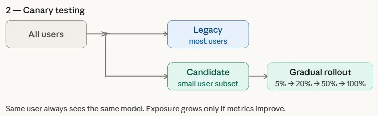
カナリアテストによる段階的ロールアウト
新モデルをまず限定的なユーザーサブセットに公開し、パフォーマンス指標が成功を示す場合にのみ徐々に公開範囲を拡大することで、早期の問題検出と迅速なロールバックを可能にする。
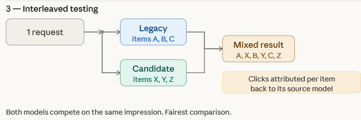
インターリーブテストとシャドウテスト
インターリーブテストは単一ユーザーセッション内で複数モデルの結果を混合提示し、シャドウテストは新モデルの推論を本番トラフィックで実行するが結果は使用せず、いずれもリスクを最小限に抑えた評価を実現する。
Interleaved Testingの仕組み
複数のモデルの出力を同じレスポンス内で混合し、ユーザーに表示することで評価する。例えばレコメンデーションシステムでは、レガシーモデルと候補モデルの両方からのアイテムをリストに含める。
Shadow Testingの特徴
本番環境で候補モデルを並行実行するが、ユーザーにはレガシーモデルの予測のみを返し、候補モデルの出力は分析用にログ記録する。実際のトラフィック下での動作を評価できるが、ユーザーエンゲージメント指標は取得できない。
シミュレーションの前提条件
各モデルはリクエストを受け取りスコアを返す関数として表現され、レガシーモデルは最大0.35、候補モデルは最大0.55のスコアを持つように設計されている。
影響分析・編集コメントを表示
影響分析
この記事は、機械学習の実運用における重要なプラクティスを体系的に整理しており、MLOpsの成熟度向上に貢献する。特に、理論と実践のギャップを埋める実用的なガイダンスを提供することで、より安全で信頼性の高いAIシステムの普及を促進する可能性がある。
編集コメント
実務志向のMLエンジニアやデータサイエンティストにとって非常に価値のある実践的ガイド。理論的なモデル開発から実際のビジネス価値創出までの橋渡しとして、具体的な戦略とその適用場面が明確に説明されている。
print("\n── 3. インターリーブテスト ──────────────────────────────────")
def interleave(pred_a, pred_b):
"""項目を交互に配置: A, B, A, B ... ソースモデルでタグ付け。"""
items_a = [("legacy", pred_a["score"] + random.uniform(-0.05, 0.05)) for _ in range(3)]
items_b = [("candidate", pred_b["score"] + random.uniform(-0.05, 0.05)) for _ in range(3)]
merged = []
for a, b in zip(items_a, items_b):
merged += [a, b]
return merged
clicks = {"legacy": 0, "candidate": 0}
shown = {"legacy": 0, "candidate": 0}
for req in requests:
pred_l = legacy_model(req)
pred_c = candidate_model(req)
for source, score in interleave(pred_l, pred_c):
shown[source] += 1
clicks[source] += int(random.random() < score) # クリック ~ スコア
for name in ["legacy", "candidate"]:
print(f" {name:12s} | インプレッション: {shown[name]:4d} "
f"| クリック: {clicks[name]:3d} "
f"| CTR: {clicks[name]/shown[name]:.3f}")
シャドウテスト
両方のモデルがすべてのリクエストを処理しますが、明確な区別があります — live_predがユーザーに返される結果であり、shadow_predは単にログに記録されるだけで、それ以上の処理は行われません。候補モデルの出力はユーザーに返されることも、表示されることも、アクションを起こされることもありません。ログリストがシャドウテストの全てです。実際のシステムでは、このログはデータベースやデータウェアハウスに書き込まれ、エンジニアが後からクエリを実行し、レガシーモデルと比較してレイテンシ分布、出力パターン、スコア分布などを分析します — すべて、1人のユーザーにも影響を与えることなく行われます。
print("\n── 4. シャドウテスト ───────────────────────────────────────")
log = [] # 候補モデルのシャドウログ
for req in requests:
# ユーザーに返される結果
live_pred = legacy_model(req)
# シャドウ実行 — ユーザーには表示されない
shadow_pred = candidate_model(req)
log.append({
"request_id": req["id"],
"legacy_score": live_pred["score"],
"candidate_score": shadow_pred["score"], # ログ記録のみ、提供されない
})
avg_legacy = sum(r["legacy_score"] for r in log) / len(log)
avg_candidate = sum(r["candidate_score"] for r in log) / len(log)
print(f" レガシーモデル 平均スコア(提供済み): {avg_legacy:.3f}")
print(f" 候補モデル 平均スコア(ログ記録): {avg_candidate:.3f}")
print(f" 注: 候補モデルのスコアにはクリック検証はありません — シャドウ実行のみです。")
完全なノートブックはこちらでチェックしてください。また、Twitterでフォローし、120k以上のメンバーが参加するML SubRedditに参加し、ニュースレターを購読することをお忘れなく。待って! Telegramをご利用ですか? 今ならTelegramでも参加できます。
この投稿「MLモデルを本番環境に安全にデプロイする方法: 4つの制御戦略(A/B、カナリア、インターリーブ、シャドウテスト)」は、MarkTechPostで最初に公開されました。
原文を表示
Deploying a new machine learning model to production is one of the most critical stages of the ML lifecycle. Even if a model performs well on validation and test datasets, directly replacing the existing production model can be risky. Offline evaluation rarely captures the full complexity of real-world environments—data distributions may shift, user behavior can change, and system constraints in production may differ from those in controlled experiments.
As a result, a model that appears superior during development might still degrade performance or negatively impact user experience once deployed. To mitigate these risks, ML teams adopt controlled rollout strategies that allow them to evaluate new models under real production conditions while minimizing potential disruptions.
In this article, we explore four widely used strategies—A/B testing, Canary testing, Interleaved testing, and Shadow testing—that help organizations safely deploy and validate new machine learning models in production environments.
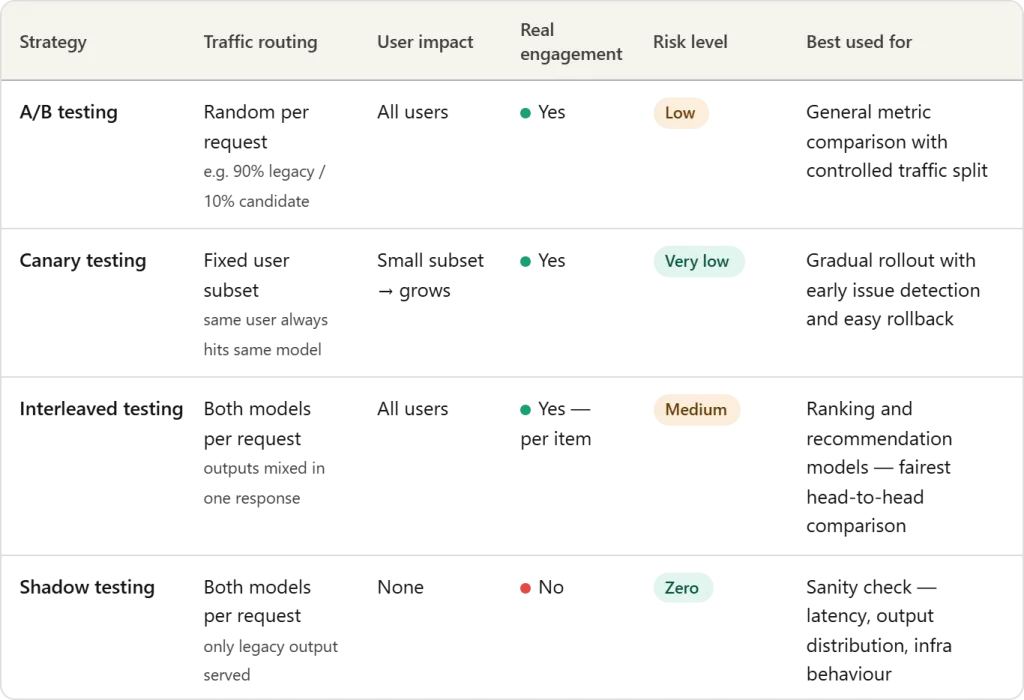
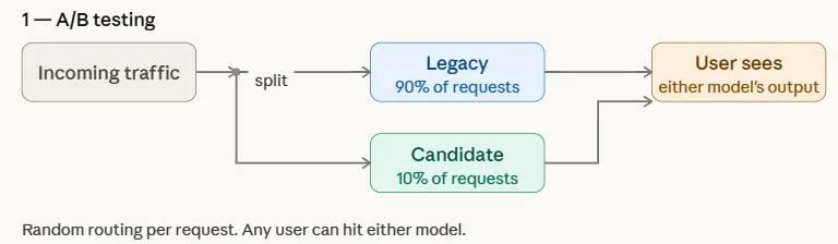
A/B Testing
A/B testing is one of the most widely used strategies for safely introducing a new machine learning model in production. In this approach, incoming traffic is split between two versions of a system: the existing legacy model (control) and the candidate model (variation). The distribution is typically non-uniform to limit risk—for example, 90% of requests may continue to be served by the legacy model, while only 10% are routed to the candidate model.
By exposing both models to real-world traffic, teams can compare downstream performance metrics such as click-through rate, conversions, engagement, or revenue. This controlled experiment allows organizations to evaluate whether the candidate model genuinely improves outcomes before gradually increasing its traffic share or fully replacing the legacy model.
Canary Testing
Canary testing is a controlled rollout strategy where a new model is first deployed to a small subset of users before being gradually released to the entire user base. The name comes from an old mining practice where miners carried canary birds into coal mines to detect toxic gases—the birds would react first, warning miners of danger. Similarly, in machine learning deployments, the candidate model is initially exposed to a limited group of users while the majority continue to be served by the legacy model.
Unlike A/B testing, which randomly splits traffic across all users, canary testing targets a specific subset and progressively increases exposure if performance metrics indicate success. This gradual rollout helps teams detect issues early and roll back quickly if necessary, reducing the risk of widespread impact.
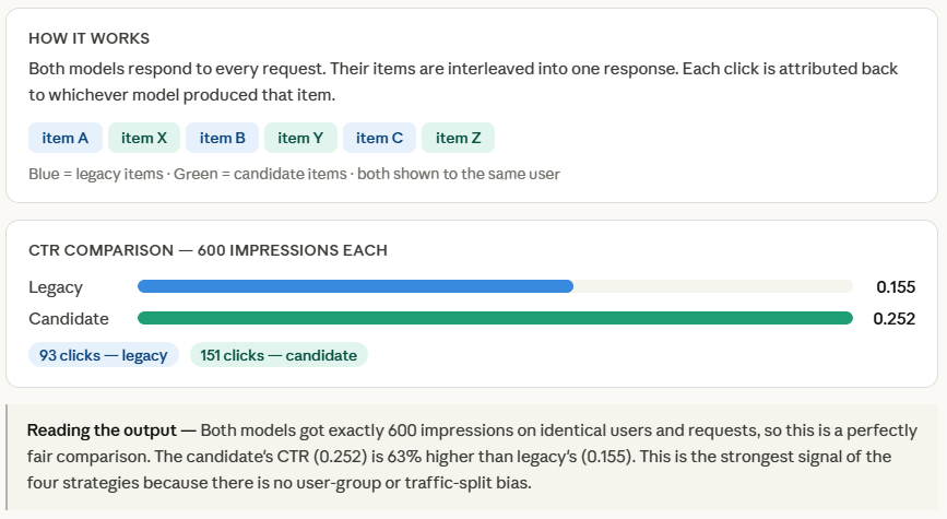
Interleaved Testing
Interleaved testing evaluates multiple models by mixing their outputs within the same response shown to users. Instead of routing an entire request to either the legacy or candidate model, the system combines predictions from both models in real time. For example, in a recommendation system, some items in the recommendation list may come from the legacy model, while others are generated by the candidate model.
The system then logs downstream engagement signals—such as click-through rate, watch time, or negative feedback—for each recommendation. Because both models are evaluated within the same user interaction, interleaved testing allows teams to compare performance more directly and efficiently while minimizing biases caused by differences in user groups or traffic distribution.
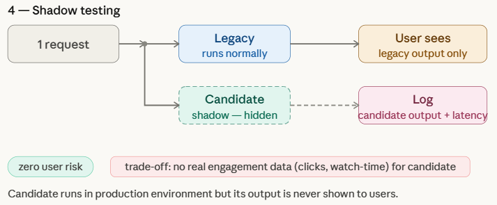
Shadow Testing
Shadow testing, also known as shadow deployment or dark launch, allows teams to evaluate a new machine learning model in a real production environment without affecting the user experience. In this approach, the candidate model runs in parallel with the legacy model and receives the same live requests as the production system. However, only the legacy model’s predictions are returned to users, while the candidate model’s outputs are simply logged for analysis.
This setup helps teams assess how the new model behaves under real-world traffic and infrastructure conditions, which are often difficult to replicate in offline experiments. Shadow testing provides a low-risk way to benchmark the candidate model against the legacy model, although it cannot capture true user engagement metrics—such as clicks, watch time, or conversions—since its predictions are never shown to users.
Simulating ML Model Deployment Strategies
Setting Up
Before simulating any strategy, we need two things: a way to represent incoming requests, and a stand-in for each model.
Each model is simply a function that takes a request and returns a score — a number that loosely represents how good that model’s recommendation is. The legacy model’s score is capped at 0.35, while the candidate model’s is capped at 0.55, making the candidate intentionally better so we can verify that each strategy actually detects the improvement.
make_requests() generates 200 requests spread across 40 users, which gives us enough traffic to see meaningful differences between strategies while keeping the simulation lightweight.
Copy CodeCopiedUse a different Browser
import random
import hashlib
random.seed(42)
def legacy_model(request):
return {"model": "legacy", "score": random.random() * 0.35}
def candidate_model(request):
return {"model": "candidate", "score": random.random() * 0.55}
def make_requests(n=200):
users = [f"user_{i}" for i in range(40)]
return [{"id": f"req_{i}", "user": random.choice(users)} for i in range(n)]
requests = make_requests()
A/B Testing
ab_route() is the core of this strategy — for every incoming request, it draws a random number and routes to the candidate model only if that number falls below 0.10, otherwise the request goes to legacy. This gives the candidate roughly 10% of traffic.
We then collect the prediction scores from each model separately and compute the average at the end. In a real system, these scores would be replaced by actual engagement metrics like click-through rate or watch time — here the score just stands in for “how good was this recommendation.”
Copy CodeCopiedUse a different Browser
print("── 1. A/B Testing ──────────────────────────────────────────")
CANDIDATE_TRAFFIC = 0.10 # 10 % of requests go to candidate
def ab_route(request):
return candidate_model if random.random() < CANDIDATE_TRAFFIC else legacy_model
results = {"legacy": [], "candidate": []}
for req in requests:
model = ab_route(req)
pred = model(req)
results[pred["model"]].append(pred["score"])
for name, scores in results.items():
print(f" {name:12s} | requests: {len(scores):3d} | avg score: {sum(scores)/len(scores):.3f}")
Canary Testing
The key function here is get_canary_users(), which uses an MD5 hash to deterministically assign users to the canary group. The important word is deterministic — sorting users by their hash means the same users always end up in the canary group across runs, which mirrors how real canary deployments work where a specific user consistently sees the same model.
We then simulate three phases by simply expanding the fraction of canary users — 5%, 20%, and 50%. For each request, routing is decided by whether the user belongs to the canary group, not by a random coin flip like in A/B testing. This is the fundamental difference between the two strategies: A/B testing splits by request, canary testing splits by user.
Copy CodeCopiedUse a different Browser
print("\n── 2. Canary Testing ───────────────────────────────────────")
def get_canary_users(all_users, fraction):
"""Deterministic user assignment via hash -- stable across restarts."""
n = max(1, int(len(all_users) * fraction))
ranked = sorted(all_users, key=lambda u: hashlib.md5(u.encode()).hexdigest())
return set(ranked[:n])
all_users = list(set(r["user"] for r in requests))
for phase, fraction in [("Phase 1 (5%)", 0.05), ("Phase 2 (20%)", 0.20), ("Phase 3 (50%)", 0.50)]:
canary_users = get_canary_users(all_users, fraction)
scores = {"legacy": [], "candidate": []}
for req in requests:
model = candidate_model if req["user"] in canary_users else legacy_model
pred = model(req)
scores[pred["model"]].append(pred["score"])
print(f" {phase} | canary users: {len(canary_users):2d} "
f"| legacy avg: {sum(scores['legacy'])/max(1,len(scores['legacy'])):.3f} "
f"| candidate avg: {sum(scores['candidate'])/max(1,len(scores['candidate'])):.3f}")
Interleaved Testing
Both models run on every request, and interleave() merges their outputs by alternating items — one from legacy, one from candidate, one from legacy, and so on. Each item is tagged with its source model, so when a user clicks something, we know exactly which model to credit.
The small random.uniform(-0.05, 0.05) noise added to each item’s score simulates the natural variation you’d see in real recommendations — two items from the same model won’t have identical quality.
At the end, we compute CTR separately for each model’s items. Because both models competed on the same requests against the same users at the same time, there is no confounding factor — any difference in CTR is purely down to model quality. This is what makes interleaved testing the most statistically clean comparison of the four strategies.
Copy CodeCopiedUse a different Browser
print("\n── 3. Interleaved Testing ──────────────────────────────────")
def interleave(pred_a, pred_b):
"""Alternate items: A, B, A, B ... tagged with their source model."""
items_a = [("legacy", pred_a["score"] + random.uniform(-0.05, 0.05)) for _ in range(3)]
items_b = [("candidate", pred_b["score"] + random.uniform(-0.05, 0.05)) for _ in range(3)]
merged = []
for a, b in zip(items_a, items_b):
merged += [a, b]
return merged
clicks = {"legacy": 0, "candidate": 0}
shown = {"legacy": 0, "candidate": 0}
for req in requests:
pred_l = legacy_model(req)
pred_c = candidate_model(req)
for source, score in interleave(pred_l, pred_c):
shown[source] += 1
clicks[source] += int(random.random() < score) # click ~ score
for name in ["legacy", "candidate"]:
print(f" {name:12s} | impressions: {shown[name]:4d} "
f"| clicks: {clicks[name]:3d} "
f"| CTR: {clicks[name]/shown[name]:.3f}")
Shadow Testing
Both models run on every request, but the loop makes a clear distinction — live_pred is what the user gets, shadow_pred goes straight into the log and nothing more. The candidate’s output is never returned, never shown, never acted on. The log list is the entire point of shadow testing. In a real system this would be written to a database or a data warehouse, and engineers would later query it to compare latency distributions, output patterns, or score distributions against the legacy model — all without a single user being affected.
Copy CodeCopiedUse a different Browser
print("\n── 4. Shadow Testing ───────────────────────────────────────")
log = [] # candidate's shadow log
for req in requests:
# What the user sees
live_pred = legacy_model(req)
# Shadow run -- never shown to user
shadow_pred = candidate_model(req)
log.append({
"request_id": req["id"],
"legacy_score": live_pred["score"],
"candidate_score": shadow_pred["score"], # logged, not served
})
avg_legacy = sum(r["legacy_score"] for r in log) / len(log)
avg_candidate = sum(r["candidate_score"] for r in log) / len(log)
print(f" Legacy avg score (served): {avg_legacy:.3f}")
print(f" Candidate avg score (logged): {avg_candidate:.3f}")
print(f" Note: candidate score has no click validation -- shadow only.")
Check out the FULL Notebook Here. Also, feel free to follow us on Twitter and don’t forget to join our 120k+ ML SubReddit and Subscribe to our Newsletter. Wait! are you on telegram? now you can join us on telegram as well.
The post Safely Deploying ML Models to Production: Four Controlled Strategies (A/B, Canary, Interleaved, Shadow Testing) appeared first on MarkTechPost.
関連記事
Anthropic、再現可能なゲノム・プロテオーム・ケミインフォマティクスパイプライン向けマルチエージェント AI ワークベンチ「Claude Science Beta」をリリース
NVIDIA HORIZON:Git ワークツリーを自律的に進化させるハンズフリーエージェントが RTL ベンチマークで完全達成
NVIDIA AI が自己改善型ロボットフレームワーク「ASPIRE」を発表、LIBERO-Pro の長期タスクでゼロショット成功率 31% を達成
今日のまとめ
AI日報で今日の重要ニュースをまとめ読み