SageMaker AI LSTMネットワークとESA STIXデータを用いた太陽フレア検出システムの構築

太陽フレアの効果的な監視と特性評価には、複数のエネルギースペクトラムにわたる X 線放出の洗練された分析が必要です。機械学習に基づく異常検知は、顕著な太陽活動を示す可能性のある重要なパターンを特定するための強力なツールです。固有の放射シグネチャを識別することで、主要な太陽事象の特徴を検出し、分析し、包括的に理解することができます。これらの検出されたパターンは、宇宙天気予報、太陽物理学調査、衛星運用計画など、さまざまな応用において不可欠です。近年、太陽監視能力は劇的に拡大し、前例のない量の X 線測定データを生成しています。このデータが継続して増加するにつれ、分析方法も進化し、これらの膨大なデータセットを効率的に処理しながら、太陽挙動における最も微妙な変動さえも捉える必要があります。高度なディープラーニングアーキテクチャ、特に Long Short-Term Memory (LSTM) ネットワークは、これらの課題に対する非常に能力の高いソリューションとして浮上しています。 本記事では、欧州宇宙機関（ESA）の X 線イメージング分光器・望遠鏡（Spectrometer/Telescope for Imaging X-rays：STIX）が収集したマルチチャネル X 線データにおける異常検出のために LSTM ニューラルネットワークを実装する方法について紹介します。当分析は、低エネルギー帯（4–10 keV）、中エネルギー帯（10–25 keV）、高エネルギー帯（25+ keV）にわたるさまざまなエネルギー範囲での異常パターンの検出を強調しています。このマルチチャネルアプローチにより、包括的な太陽活動の監視が可能となり、X 線放出データの洗練されたパターン分析を通じて、潜在的なフレア事象を堅牢に特定することが可能になります。本記事では、ESA の STIX 装置からのデータを用いて太陽フレアを検出するためのディープラーニングモデルを構築・デプロイする方法を [Amazon SageMaker AI](https://aws.amazon.com/sagemaker/ai/) を使って解説します。SageMaker AI は、データの密度とスパースシティ（sparsity：疎性）に基づいて異常スコアを割り当てることで異常なデータポイントを検出する教師なし学習アルゴリズムであるランダムカットフォレスト（Random Cut Forest：RCF）を利用します。また、マルチチャネル X 線データを処理して潜在的な太陽フレア事象を特定するロングショートタームメモリー（Long Short-Term Memory：LSTM）ニューラルネットワークの実装方法についても学びます。 ## 主要概念 このセクションでは、本ソリューションにおける太陽放射分析および機械学習（ML）のいくつかの主要概念について議論します。 ## ソーラー観測における X 線エネルギーチャネル STIX データ内の X 線放出は、低エネルギー（4–10 keV）、中エネルギー（10–25 keV）、高エネルギー（25+ keV）の複数のエネルギーバンドにわたって測定されます。このマルチチャネルアプローチにより、異なるエネルギーレベルにおける太陽活動の包括的なモニタリングが可能になります。エネルギーバンドは、太陽フレアの発生から最大強度に至るまでのさまざまな側面に関する重要な情報を提供します。これらのチャネル全体のパターンを分析することで、太陽フレアの進化の異なる段階を特定し、その強度を特徴づけることができます。 複数のエネルギーチャネルからのデータを組み合わせることで、太陽フレアの特徴に関する詳細な洞察が得られます。高エネルギーチャネルは通常、より激しいフレア活動を示す一方、低エネルギーチャネルでは前兆事象やフレア後の現象を捉えることができます。このマルチスペクトルアプローチにより、フレアの発生を早期に検知し、フレアの規模と持続時間を正確に評価することが可能になります。 ## 宇宙機ダイナミクスにおける四元数 LSTM ネットワークは、時系列データ内の長期的な依存関係を捉えることができる内部メモリ状態を維持する点で、従来のニューラルネットワークとは異なります。この独自の性質により、それは再帰型ニューラルネットワーク（RNN: Recurrent Neural Network）の一種として位置づけられ、その [バリアント](https://aws.amazon.com/what-is/recurrent-neural-network/) となっています。LSTM の能力は、パターンが長い期間にわたって発展する可能性がある太陽フレア検出において特に価値があります。 LSTM アーキテクチャは、ゲートと状態の複雑なシステムを通じて動作します。その中核には、新しい情報のネットワークへの流れを制御する入力ゲートがあり、どのデータポイントが保存に値する重要なものかを決定します。これと並行して機能する忘却ゲートは既存情報を評価し、どの要素を廃棄すべきかを判断することで、無関係なデータの蓄積を防ぎます。これらの決定はセル状態に反映され、これはネットワークの長期記憶として機能し、シーケンス処理を通じて重要な情報を維持します。その後、出力ゲートが、このセル状態からのどの情報が各タイムステップで出力として提示されるべきかを調節します。 この洗練されたアーキテクチャにより、モデルは異なるエネルギーチャネル間の複雑な関係を学習しながら、分析における時間的整合性を維持できます。多層アプローチによってネットワークはデータのより抽象的な表現を構築し、正則化技術が新しい観測データに対する信頼性の高い性能を保証します。予測値と実際の値の間の再構成誤差を継続的に監視することで、システムは太陽フレア事象を示す可能性のある異常パターンを効果的に特定します。 ## 時系列解析と異常検出 異常検出システムは、各次元が異なるエネルギーチャネルに対応する多次元時系列データを処理します。LSTM モデルは X 線放出データの通常のパターンを学習し、太陽フレア事象を示す可能性のある逸脱を検出します。これらの異常は、急激な強度の増加、異常なスペクトルパターン、または太陽活動の他の兆候を表している可能性があります。 信頼性の高いフレア検出のため、LSTM はクロスチャネル X 線データの時間的およびスペクトルの両方の特性を分析します。時間解析は、時間の経過に伴う放出強度における急激な変化や異常パターンの特定に焦点を当てています。一方、スペクトル解析は、異なるエネルギーチャネル間の関係を調べます。太陽フレアはしばしば複数のエネルギー帯域にわたって特徴的なパターンを生み出すためです。 LSTM に基づくパターン認識とマルチチャネル分析の組み合わせにより、自動化された太陽フレア検出のための堅牢なフレームワークが構築されます。このアプローチは、微妙な前兆パターンの特定、フレアの進化の追跡、および異なるエネルギー範囲にわたるフレア強度の特徴付けを可能にし、宇宙天気予報や太陽物理学研究にとって貴重な洞察を提供します。 ## ソリューションアーキテクチャ 本ソリューションは、以下の図に示すように、ESA Solar Orbiter の太陽 STIX データに対して [LSTM アルゴリズム](https://docs.aws.amazon.com/sagemaker/latest/dg/rcf_how-it-works.html) を用いた異常検出を実装しています。このソリューションでは、Amazon SageMaker AI と共に Bring Your Own Script (BYOS) を採用しており、SageMaker AI の管理されたインフラストラクチャを活用しながら、独自のトレーニングスクリプトを使用することが可能です。BYOS を利用することで、以下のことが実現できます。 - 好みの機械学習フレームワーク（本ケースでは PyTorch）の使用 - トレーニングロジックに対する完全な制御の維持 - SageMaker AI のトレーニングインフラストラクチャとスケーリング機能の継続的な活用 - コンテナ管理を行わずに、独自の LSTM モデルを展開 このアプローチを利用するには、Python スクリプトを SageMaker AI にアップロードし、トレーニングジョブを作成する際にエントリポイントとして指定します。本ブログ記事で使用されている Python コードは、参照されている [GitHub リポジトリ](https://github.com/aws-samples/sample-sagemaker-ai-lstm-anomaly-detection-solar-flare) 内に格納されています。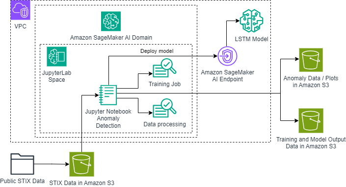 ![image](https://d2908q01vomqb2.cloudfront.net/f1f836cb4ea6efb2a0b1b99f41ad8b103eff4b59/2026/03/24/ML-19354-1.png) データパイプラインは、FITS形式で保存された生のSTIX（Spectrometer/Telescope for Imaging X-rays）測定値から開始します。これらの観測データは、主要な開発および分析プラットフォームとして機能するJupyterLab環境内で初期処理が行われます。この環境には、FITSデータをCSV形式へ変換し、高度な検出アルゴリズムを実行するためのカスタムPythonノートブックが格納されています。 システムの核心を担うのは、ニューラルネットワークによる処理パイプラインです。ワークフローはJupyterLabでのデータ準備から始まり、PyTorchで実装された専用のCrossChannelLSTMモデルのトレーニングへと進みます。このモデルは、複数のエネルギー範囲（4–10 keV、10–25 keV、および25+ keV）にわたるX線放射を処理します。トレーニングフェーズの後、システムは時系列データを分析し、異常検出を通じて潜在的な太陽フレアの兆候を特定します。パイプラインの最終段階では、包括的な可視化が生成され、これには時系列分析プロット、エネルギー進化図、およびチャネル間相関表示が含まれます。 本システムは、特定された異常値、詳細なチャネル統計情報、および時系列パターン分析を含む広範な解析出力を生成します。可視化スイートでは、エネルギー帯域全体にわたる異常パターンを強調した複雑なプロットが作成され、これには時系列の推移を示すチャートやモデルのパフォーマンス指標も含まれています。すべての発見結果は、異常インジケーターと再構成誤差測定値を含む構造化された CSV ファイルに文書化されており、検出された太陽事象の詳細な分析を可能にします。プロセス全体を通じて、厳格なデータ処理プロトコルが解析の整合性と再現性を維持します。 ## ソリューションの概要 このソリューションは、深層学習技術を用いた太陽フレア検出のための包括的なアプローチを示しています。まず、STIX のクイックルック光曲線データを含む FITS ファイル形式のデータを扱いやすい CSV 形式に変換するデータ前処理を行います。次に、分析のための高品質な入力データを維持するために、データの正規化とシーケンス準備を実施します。PyTorch を用いて、マルチチャネル X 線データにおける異常を検出するために特別に設計されたカスタム CrossChannelLSTM モデルを実装します。本システムは複数のエネルギー帯域にわたってデータを処理し、太陽フレア活動を示す可能性のあるパターンを特定します。 モデルのトレーニングフェーズ（ドロップアウト正則化を備えた複数の LSTM レイヤーを使用）が完了した後、このソリューションは広範な可視化機能を提供します。これには、異常を強調表示した時系列プロット、エネルギーと時間の進化を示す可視化、および結果を明確に解釈するためのチャネル間分析プロットが含まれます。システムは、チャネル固有の統計情報、異常の時系列的な進化、および異常フラグと再構成誤差を含む包括的な CSV ファイルなど、詳細な出力を生成します。 この深層学習アーキテクチャと可視化ツールの組み合わせは、自動太陽フレア検出のための堅牢なフレームワークを構築します。この組み合わせにより、迅速な検出と精密な分析が不可欠な宇宙天気監視アプリケーションに特に適しています。大規模な STIX データを処理しながら微妙な放射パターンを特定する能力は、太陽物理学研究および宇宙天気予報におけるその有効性を示しています。 ## 前提条件 太陽フレア検出システムを実装する前に、以下のツールと依存関係がインストールされていることを確認してください。 - AWS の要件: 適切な権限を持つ AWS アカウント - 適切な SageMaker AI および Amazon Simple Storage Service (Amazon S3) アクセスポリシーを付与された IAM ロール - データおよびモデルアーティファクトの保存用の Amazon S3 バケット - 必要な AWS サービス: Amazon SageMaker AI (ml.m5.2xlarge JupyterLab インスタンスを推奨) - Amazon S3 - AWS IAM Identity Center - 開発環境には Python 3.7 以降が必要であり、提供された Python スクリプトおよび要件ファイルに含まれる必須の Python パッケージも用意する必要があります: - JupyterLab 環境の場合: Amazon SageMaker AI Studio のノートブック - その他の要件: FITS フォーマットの STIX データへのアクセス権限 - 大規模データの処理に必要な十分な RAM (推奨最小値は 16GB) - モデル学習の高速化には GPU サポートを推奨 - Python プログラミングおよびディープラーニングの基本概念に関する基本的な理解 - 推定コスト: SageMaker AI ml.m5.4xlarge インスタンス: 時間あたり約 $0.922 - S3 ストレージ: GB あたり月間約 $0.023 - このソリューションを実行するための総推定コスト: 数時間の試行実験で約 $10〜$15 ## ソリューションのセットアップ セットアッププロセスには、すべてのデータ分析およびモデル学習が実行される Amazon SageMaker AI Python 環境の設定が含まれます。 - Amazon SageMaker AI コンソールで、SageMaker AI ドメインの詳細ページを開きます。 - JupyterLab を開き、このプロジェクト用の新しい Python ノートブックインスタンスを作成します。 - 環境の準備が整ったら、Amazon SageMaker AI JupyterLab のターミナルを開き、以下のコマンドを使用してプロジェクトリポジトリをクローンします： git clone https://github.com/aws-samples/sample-SageMaker-ai-lstm-anomaly-detection-solar-orbiter.git cd sample-SageMaker-ai-lstm-anomaly-detection-solar-orbiter - 必要な Python ライブラリをインストールします： pip install -r requirements.txt このプロセスにより、Solar Orbiter センサーデータに対する異常検出分析を実行するための必要な依存関係が設定されます。 ## 異常検出の実行 スクリプト内の bucket_name および file_name 変数を、ご自身の S3 バケット名とデータファイル名に更新してください。 JupyterLab で Jupyter ノートブックとしてスクリプトを実行するか、Python スクリプトとして実行します： python ESA_SolOrb_AD.py 実行すると、ノートブックまたはスクリプトは太陽 X 線データを分析するための一連の自動化タスクを実行します。まず、FITS ファイルを読み込んで前処理を行い、CSV 形式に変換してエネルギーチャネル間でデータを正規化します。次に、PyTorch を使用して CrossChannelLSTM モデルをトレーニングし、異常検出システムの基盤を構築します。モデルが稼働すると、多チャネルの X 線データを処理し、異なるエネルギーバンド（4–10 keV、10–25 keV、および 25+ keV）にわたるパターン分析を通じて、潜在的な太陽フレア事象を特定します。 ## コード構造 Python の実装は、[main スクリプト](https://github.com/aws-samples/sample-sagemaker-ai-lstm-anomaly-detection-solar-flare/blob/main/ESA_SolOrb_AD.py)を中心に構成された太陽フレア検出パイプラインを中核としています。その核心には、CrossChannelLSTM と CrossChannelDataset という 2 つの主要なクラスがあり、これらがデータ取り込みから可視化までのワークフローを連携して実行します。これらのクラスは協調して STIX X 線データを処理し、潜在的な太陽フレア事象を特定します。 explore_ql_lightcurve メソッドは、初期のデータ取り込みと前処理を担当し、FITS ファイルを CSV 形式に変換して、分析のために X 線測定値が適切にフォーマットされるように保証します。plot_lightcurve メソッドは、異なるエネルギーチャネルにわたるデータの初期可視化を作成します。print_channel_stats メソッドは、各エネルギーバンドに対する統計分析を提供します。 CrossChannelLSTM クラスは、複数の LSTM レイヤーとドロップアウト正則化を備えたニューラルネットワークアーキテクチャを実装しています。CrossChannelDataset クラスは、モデルのためのデータ準備とシーケンシングを管理します。その後、detect_cross_channel_anomalies メソッドはこの訓練済みモデルを使用して、異なるエネルギーバンドにおける X 線放出の異常パターンを特定します。 可視化のため、plot_cross_channel_anomalies および plot_flare_anomalies メソッドは、検出された異常、時間的進化パターン、およびエネルギーバンド分布を強調した詳細なグラフを作成します。これらの可視化には、時系列分析、エネルギー - 時間進化図、クロスチャネル相関プロットが含まれます。 これらすべてのコンポーネントが組み合わさることで、マルチチャンネル X 線データを処理し、さらなる調査が必要な太陽フレア事象を特定するための包括的なパイプラインが構築されます。システムのモジュール型設計により、特定の分析ニーズに合わせてモデルパラメータや可視化オプションを変更することが可能です。 ## 設定 スクリプト内の以下のパラメータは、精度、パフォーマンス、計算時間、その他の要件に応じた適切な使用のために必要に応じて調整してください：LSTM モデルのアーキテクチャとトレーニングパラメータは、太陽フレア事象の検出に大きな影響を与えます。 以下の変更が可能です： モデルアーキテクチャパラメータ： - hidden_size: LSTM の隠れ層のサイズ（デフォルト：128–256） - num_layers: LSTM レイヤーの数（デフォルト：2–3） - dropout_rate: ドロップアウト正則化率（デフォルト：0.2） - sequence_length: 入力シーケンスの長さ（デフォルト：30–50） トレーニングパラメータ: - batch_size: トレーニングバッチあたりのシーケンス数（デフォルト：32） - num_epochs: トレーニング反復回数（デフォルト：15–20） - learning_rate: モデルパラメータの更新率（デフォルト：0.001） - threshold_multiplier: 異常検出感度（デフォルト：1.5） 標準的なハードウェア構成でのパフォーマンス向上には、以下の設定を推奨します: - hidden_size=256 - num_layers=3 - dropout_rate=0.2 - sequence_length=30 - batch_size=32 - num_epochs=20 ハードウェア要件はトレーニング時間とモデルのパフォーマンスに大きな影響を与えます。高速なトレーニングには GPU 加速が推奨されますが、CPU のみの実行もサポートされています。最小推奨システム仕様として、16 GB の RAM と 4 つの CPU コアを挙げます。 本システムでは、可視化パラメータと出力形式のカスタマイズが可能です。結果は、各エネルギーチャネルの詳細な異常フラグと再構成誤差を含む CSV ファイルとして保存できます。可視化スイートは、時系列プロットからエネルギーバンド分布まで、分析の異なる側面を表示するように設定可能です。 ## データ 本スクリプトは、FITS ファイル形式の [ESA Solar Orbiter STIX（X 線イメージング分光計・望遠鏡）公開データ](https://soar.esac.esa.int/soar/) を使用します。このデータには、4 keV から 25 keV を超える範囲にわたる複数のエネルギーチャネルにおける X 線の測定値が含まれています。FITS ファイルには以下の情報が含まれます： - エネルギーチャネルごとの時系列データ - エネルギーバンド情報（4–10 keV、10–25 keV、25+ keV） - コントロールインデックスおよびタイミング情報 - 測定誤差データ

SageMaker AI LSTMネットワークとESA STIXデータを用いた太陽フレア検出システムの構築

背景や根拠まで確認しますか？

調べる

選ぶ

サイト